15. Matrix decomposition#
Saleh Rezaeiravesh, saleh.rezaeiravesh@manchester.ac.uk
Department of Mechanical and Aerospace Engineering, The University of Manchester, Manchester, UK
15.1. Intended Learning Outcomes#
After reading and running this notebook, the students should be able to:
Use
numpyandscipybuilt-in functions to do matrix deccomposition including Cholesky, QR, and LU decompositions.Implement relevant algorithms to develop Python functions to do the above decompositions.
15.2. Import libraries#
numpy.linalg provides built-in functions for Cholesky and QR decomposition. However, for the LU decomposition, we need to use the built-in function from another Python package, scipy.linalg. Note that scipy that is a package for “fundamental algorithms for scientific computing in Python”.
import numpy as np
import numpy.linalg as la
import scipy.linalg as sc
15.3. Cholesky decomposition#
Assume \(\mathbf{C}\) is a Hermitian positive definite square matrix. If all elements are real, then \(\mathbf{C}\) is a symmetric positive definite matrix. This is the case that we deal within this unit.
Recall:
A square matrix \(\mathbf{C}\) is Hermitian, if \(\mathbf{C} = \bar{\mathbf{C}}^T\), i.e. \(c_{ij} = \bar{c}_{ji}\) for \(i,j=1,2,\cdots,n\). Here \(\bar{c}_{ji}\) is the complex conjugate of \(c_{ji}\).
A real square matrix \(\mathbf{C}\) is Hermitian, if \(\mathbf{C} =\mathbf{C}^T\), i.e \(\mathbf{C}\) is symmetric.
A square matrix \(\mathbf{C}\) is positive definite if all its eignvalues are positive.
By Cholesky decomposition, \(\mathbf{C}\) is decomposed into a lower-triangular matrix \(\mathbf{L}\), such that:
where,
Example: Check if the following matrix is Hermitian positive definite square, and hence can be decomposed by the Cholesky method.
C = np.array([[4,-12,16],[-12,37,-43],[16,-43,98]])

print(C)
[[  4 -12  16]
 [-12  37 -43]
 [ 16 -43  98]]
This matrix is symmetric, since \(\mathbf{C}=\mathbf{C}^T\). Now let’s find its eigenalues:
eigVals, eigVecs = la.eig(C)
print(eigVals)
[1.23477232e+02 1.88049805e-02 1.55039632e+01]
All its eigen values are positive, so \(\mathbf{C}\) is positive definite. Therefore, \(\mathbf{C}\) fulfills all conditions required by the Cholesky decomposition.
15.3.1. numpy built-in function#
To perform the Cholesky decomposition of a Hermitian positive definite square matrix \(\mathbf{C}\), we can use the built-in function L = numpy.linalg.cholesky(C). This returns \(\mathbf{L}\), a lower triangular matrix:
L = la.cholesky(C)  #returns lower triangular matrix
print(L)
[[ 2.  0.  0.]
 [-6.  1.  0.]
 [ 8.  5.  3.]]
We can check if the docomposition works as it should by computing \(\mathbf{L}\mathbf{L}^T\) that has to be numerically equal to the original matrix \(\mathbf{C}\):
C2 = L @ L.T   #reconstruced C from L

dC = C - C2    #The difference between the original C and reconstructed C
print(dC)
[[0. 0. 0.]
 [0. 0. 0.]
 [0. 0. 0.]]
This confirms that \(\mathbf{C} = \mathbf{L}\mathbf{L}^T\) holds.
15.3.2. Direct implementation#
Now, instead of using the numpy.linalg built-in function, we want to write a Python function implementing the above formula to compute \(\ell_{ij}\) for \(i,j=1,2,\cdots,n\) and create the lower triangular matrix \(\mathbf{L}\).
def choleskyDecomp(C):
    """
    Creates a lower triangular matrix L from input matrix C that should be symmetric positive definite square.
    """
    #Check if C is square and two-dimensional
    if C.shape[0] != C.shape[1] or C.ndim !=2:
       raise ValueError("C must be a 2D symmetric matrix!")

    #Check if C is symmetric
    if not np.allclose(C,C.T):
       raise ValueError("C must be symmetric!")

    #Check if C is positive definite
    eigVals, eiVecs = la.eig(C)    #find the eigenvalues of C
    for eig_ in eigVals:
        if eig_ < 0:               #returns error if any of the eigenvalues of C is negative
           raise ValueError("C must be positive definite!")

    #compute L, the lower triangular matrix, s.t. C = L L^T
    n = C.shape[0]   #size of C in each of its two dimensions
    L = np.zeros((n,n))   #initialize L

    for i in range(n):
        for j in range(i+1):
            s = np.dot(L[i,:i], L[j,:i])

            L[i,i] = np.sqrt(C[i,i] - s)
            L[i,j] = (C[i,j] - s)/L[j,j]

    return L
L = choleskyDecomp(C)
The resulting \(\mathbf{L}\) from our function is the same as the output of numpy.linalg.cholesky(C):
print(L)

L1 = la.cholesky(C)
print(L1)
[[ 2.  0.  0.]
 [-6.  1.  0.]
 [ 8.  5.  3.]]
[[ 2.  0.  0.]
 [-6.  1.  0.]
 [ 8.  5.  3.]]
15.4. QR decomposition#
Assume \(\mathbf{E}\) is a real square matrix. Then it can be decomposed as,
where,
\(\mathbf{Q}\) is an orthogonal matrix, i.e. \(\mathbf{Q}^T = \mathbf{Q}^{-1}\).
\(\mathbf{R}\) is an upper triangular matrix.
15.4.1. numpy built-in function#
In numpy.linalg we use Q,R = qr(E):
E = np.array([[3,-5,6],[9,4,7],[-2,5,-1]])
print(E)
[[ 3 -5  6]
 [ 9  4  7]
 [-2  5 -1]]
Q,R = la.qr(E)
print('Q=', Q)
print('R=',R)
Q= [[-0.30942637  0.66518914  0.67954303]
 [-0.92827912 -0.36631688 -0.06410783]
 [ 0.20628425 -0.65064226  0.73082929]]
R= [[-9.69535971 -1.13456337 -8.56079634]
 [ 0.         -8.04442453  2.07755892]
 [ 0.          0.          2.89767405]]
Now, let’s check if the orthogonality of \(\mathbf{Q}\) holds numerically, i.e. if \(\mathbf{Q}^{-1}=\mathbf{Q}^{T}\):
Q_inv = la.inv(Q)
Q_t = Q.T
print('inv(Q)-Q.T = ',Q_inv-Q_t)
inv(Q)-Q.T =  [[-2.22044605e-16 -2.22044605e-16 -2.77555756e-17]
 [-4.44089210e-16  2.22044605e-16  2.22044605e-16]
 [ 1.11022302e-16  1.52655666e-16  1.11022302e-16]]
15.4.2. Householder Triangularization Algorithm#
We can alternatively implement Householder Triangularization Algorithm in numpy to find QR decomposition of a matrix. The algorithm is given below:
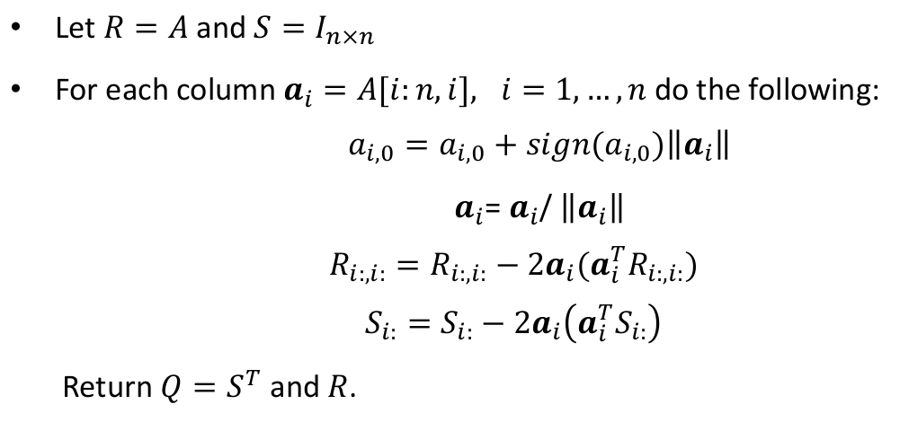
The following function implements the above algorithm:
def QR_Householder(A):
    """
    QR Decomposition based on Householder Triangularization
    """
    n = A.shape[0]
    R = A
    Q = np.identity(n)
    for k in range(n-1):
        u = np.copy(R[k:,k])

        u[0] = u[0]+np.sign(u[0])*la.norm(u)

        u = u/la.norm(u)

        #tmp=2.*u[:,None] @ (u @ R[k:,k:])[None,:]   #an alternative to the next line
        tmp=2.*np.outer(u , (u @ R[k:,k:]))
        R[k:,k:] = R[k:,k:] - tmp

        #tmp2 = 2.*u[:,None] @ (u @ Q[k:])[None,:]   #an alternative to the next line
        tmp2 = 2.*np.outer(u , (u @ Q[k:]))
        Q[k:] = Q[k:] - tmp2

    Q = Q.T
    return Q,R
Let’s test the above function
A = np.array([[3.,-5.,6.],[9.,4.,7.],[-2.,5.,-1.]])
Q,R = QR_Householder(A)
The values given by numpy built-in function are:
Q_numpy,R_numpy = la.qr(A)
print(Q)
print(Q_numpy)
[[-0.30942637  0.66518914  0.67954303]
 [-0.92827912 -0.36631688 -0.06410783]
 [ 0.20628425 -0.65064226  0.73082929]]
[[1. 0. 0.]
 [0. 1. 0.]
 [0. 0. 1.]]
print(R)
print(R_numpy)
[[-9.69535971 -1.13456337 -8.56079634]
 [ 0.         -8.04442453  2.07755892]
 [ 0.          0.          2.89767405]]
[[-9.69535971 -1.13456337 -8.56079634]
 [ 0.         -8.04442453  2.07755892]
 [ 0.          0.          2.89767405]]
15.5. LU Decomposition#
Let \(\mathbf{A}\) be an \(n\times n\) matrix. By LU decomposition, \(\mathbf{A}\) is written as the multiplication of a lower triangular matrix \(\mathbf{L}\) and an upper triangular matrix \(\mathbf{U}\) (both are \(n\times n\)):
There is no command available in numpy.linalg for LU factorisation. Instead, we can use a built-in function from another Python package, scipy: P,L,U = scipy.linalg.lu(A), where P is a permutation matrix.
If \(\mathbf{A}\) is diagonally dominant, the \(\mathbf{P}=\mathbf{I}\). Therefore, \(\mathbf{A}=\mathbf{LU}\).
Otherwise, \(P\neq I\); then, \(\mathbf{A}=\mathbf{PLU}\).
\(\mathbf{P}\) corresponds to the partial pivoting to reorder rows/columns of \(\mathbf{A}\) to achieve diagonal dominance. This is what we do in the Gaussian elimination method to solve systems of linear equations, see this notebook.
Example: LU decomposition of a diagonally dominant matrix.
A = np.array([[6.,1.,3.],[-6.,8.,-1.],[0.,0.,-17.]])

print(A)

P, L,U = sc.lu(A)
[[  6.   1.   3.]
 [ -6.   8.  -1.]
 [  0.   0. -17.]]
print("P, L, U:")
print(P)
print(L)
print(U)
P, L, U:
[[1. 0. 0.]
 [0. 1. 0.]
 [0. 0. 1.]]
[[ 1.  0.  0.]
 [-1.  1.  0.]
 [ 0.  0.  1.]]
[[  6.   1.   3.]
 [  0.   9.   2.]
 [  0.   0. -17.]]
We can reconstruct \(\mathbf{A}=\mathbf{LU}\):
#reconstructed A
print(L @ U)

#original A
print(A)
[[  6.   1.   3.]
 [ -6.   8.  -1.]
 [  0.   0. -17.]]
[[  6.   1.   3.]
 [ -6.   8.  -1.]
 [  0.   0. -17.]]
Example: LU decomposition of a non-diagonally dominant matrix.
A = np.array([[1.,-5.,6.],[9.,4.,7.],[-2.,5.,-1.]])

P, L,U = sc.lu(A)
print("P, L, U:")
print(P)
print(L)
print(U)
P, L, U:
[[0. 0. 1.]
 [1. 0. 0.]
 [0. 1. 0.]]
[[ 1.          0.          0.        ]
 [-0.22222222  1.          0.        ]
 [ 0.11111111 -0.9245283   1.        ]]
[[9.         4.         7.        ]
 [0.         5.88888889 0.55555556]
 [0.         0.         5.73584906]]
Reconstruct \(\mathbf{A}\) as \(\mathbf{A}=\mathbf{PLU}\):
#reconstructed A
print(P @ L @ U)

#original A
print(A)
[[ 1. -5.  6.]
 [ 9.  4.  7.]
 [-2.  5. -1.]]
[[ 1. -5.  6.]
 [ 9.  4.  7.]
 [-2.  5. -1.]]