5. Arrays in numpy#
Saleh Rezaeiravesh, saleh.rezaeiravesh@manchester.ac.uk
Department of Mechanical and Aerospace Engineering, The University of Manchester, Manchester, UK
https://numpy.org/doc/stable/user/absolute_beginners.html.
5.1. Intended Learning Outcomes:#
By reading and running this notebook, the students should be able to:
Define arrays of any shape in
numpy.Understand the indices, slicing, and special arrays in Python.
Use
numpyto perform basic operations on arrays.
5.2. Import numpy#
At the beginning of any .py script or Jupyter notebook, we import numpy to have access to different classes, functions, and attributes within it. The imported library can also be named by an abbreviation, for instance np.
import numpy as np
5.3. Define an array#
Within this course, we only consider the arrays of numbers. The mathematical correspondence to these arrays are tensors. As we know, a zero-order tensor is a scalar, a first-order tensor is a vector, and higher-order tensors are usually referred to as matrices. In the following cells, we provide a few examples for defining arrays in numpy. For this purpose we use numpy.array([...]), where an array’s elements (separated by a comma) are defined within the brackets [ ].
5.3.1. 1D Arrays (vectors)#
Let’s define \(\mathbf{x}_1=[-1.5,3,5,7.4]\) that is a vector of size 4:
x1 = np.array([-1.5,3,5,7.4])
Print the array:
print(x1)
[-1.5 3. 5. 7.4]
For any array defined in numpy, we can get the dimension, size, and shape of the array using the following attributes:
Dimension:
ndimShape:
shapeSize:
size
Also, we can also use Python native function len() to find the size of a 1D array (similar to lists, tuples, etc).
Let’s apply this to x1 array defined above:
print('dimension:',x1.ndim)
print('shape:',x1.shape)
print('size:',x1.size)
print('length:',len(x1))
dimension: 1
shape: (4,)
size: 4
length: 4
Note: In contrast to Matlab, a 1D array in Python has the shape, here, (4,) and not (4,1).
To reshape x1 to the latter that is a 2D array (matrix), we can do the following:
x2 = x1[:,None]

print(x2)
print('dimension:',x2.ndim)
print('shape:',x2.shape)
print('size:',x2.size)
print('length:',len(x2))
[[-1.5]
 [ 3. ]
 [ 5. ]
 [ 7.4]]
dimension: 2
shape: (4, 1)
size: 4
length: 4
Note that now, each element of the array is within a pair of brackets.
5.3.2. 2D Arrays (2D Matrices)#
We are familiar with 2D arrays or matrices that can be square or non-square, for instance:
Again we use numpy.array to define these in Python.
A1 = np.array([[-1,3,4], [2,-5,7]])
A2 = np.array([[-1,3,4], [2,-5,7], [0,6,8]])
Every row of the mathematical matrices are defined within the internal square brackets separated by a comma. The outermost brackets specify the whole matrix.
We can print these arrays along with their dimension, size, and shape:
print(A1)
print('dimension, size, shape of A1: ',A1.ndim,A1.size,A1.shape)
[[-1  3  4]
 [ 2 -5  7]]
dimension, size, shape of A1:  2 6 (2, 3)
print(A2)
print('dimension, size, shape of A2: ',A2.ndim,A2.size,A2.shape)
[[-1  3  4]
 [ 2 -5  7]
 [ 0  6  8]]
dimension, size, shape of A2:  2 9 (3, 3)
These show that,
A1is a 2D array (matrix) of shape \(2\times 3\) with \(6\) elements, in total.A2is a 2D array (matrix) of shape \(3\times 3\) with \(9\) elements, in total.
Note: The shape of an array is also an array, where the value in each of its dimension specifies the number of elements of the original array in the same direction:
A1_shape = A1.shape
print(A1_shape)
print(A1_shape[0],A1_shape[1])
(2, 3)
2 3
Note You can use len(A) to find the dimension of a multidiemnsional array:
print(len(A1))
print(A1.ndim)
2
2
5.3.3. Data type#
In some of the above examples, we defined elements of arrays as integer. This may lead to inaccuracies (due to precision) if such arrays are to be used in some numerical operations.
In such case, we can convert the type of the elements from integer to float, by explicitly setting dtype=float when defining an array.
For instance, let’s consider the 2D array \(A_1\) defined above.
A1 = np.array([[-1,3,4], [2,-5,7]])

print(A1)
print(A1.dtype)
[[-1  3  4]
 [ 2 -5  7]]
int64
As you see, A1.dtype returns int64 as the type of all elements. To define the array’s elements as 64-bit floating point numbers, we use dtype=float:
A1 = np.array([[-1,3,4], [2,-5,7]], dtype=float)
print(A1)
print(A1.dtype)
[[-1.  3.  4.]
 [ 2. -5.  7.]]
float64
An alternative way is to use . or .0 when defining the elements at the first place:
A1 = np.array([[-1.,3.,4.], [2.,-5.,7.]])
print(A1)
print(A1.dtype)
[[-1.  3.  4.]
 [ 2. -5.  7.]]
float64
5.3.4. Array initialization#
In some cases in Python codes, we need to initialize arrays of known sizes. For this, we use commands zeros and ones similar to Matlab, which lead to arrays with all elements equal to 0.0 and 1.0, respectively. Clearly, we can premultiply an array defined by ones by a scalar to have elements equal to that scalar.
Define 1D arrays:
y1 = np.zeros(5)

print(y1)
[0. 0. 0. 0. 0.]
y2 = 3.2 * np.ones(6)

print(y2)
[3.2 3.2 3.2 3.2 3.2 3.2]
Define a 2D array of shape \(4\times 3\) with all elements being 0.0:
B1=np.zeros((4,3))

print(B1)
print(B1.shape)
[[0. 0. 0.]
 [0. 0. 0.]
 [0. 0. 0.]
 [0. 0. 0.]]
(4, 3)
5.3.5. Value assignment#
The elements of a numpy array can be updated manually or through operations. For the former, simply assign a value to a specific element or a set of elements using corresponding index or index range, respectively (see below for more information about indices).
Consider the 1D array y2 defined above:
print(y2)
[3.2 3.2 3.2 3.2 3.2 3.2]
Let’s update the 4th element of the array to 5.8 and print the resulting array:
y2[3] = 5.8
print(y2)
[3.2 3.2 3.2 5.8 3.2 3.2]
We can set the 5-th elements and all subsequent elements to -1.5:
y2[4:] = -1.5
print(y2)
[ 3.2 3.2 3.2 5.8 -1.5 -1.5]
The same updating can be applied to the elements of multidimensional arrays. Below, we update all elements of B1 from the 2nd row and up to the 2nd column.
# 2D array
print(B1)

B1[1:,:2] = 1.5

print(B1)
[[0. 0. 0.]
 [0. 0. 0.]
 [0. 0. 0.]
 [0. 0. 0.]]
[[0.  0.  0. ]
 [1.5 1.5 0. ]
 [1.5 1.5 0. ]
 [1.5 1.5 0. ]]
A single element of a 2D array can also be updated similar to a 1D array:
B1[2,0] = 5.0
print(B1)
[[0.  0.  0. ]
 [1.5 1.5 0. ]
 [5.  1.5 0. ]
 [1.5 1.5 0. ]]
5.4. Indices, Slices, and Axes#
5.4.1. Indices#
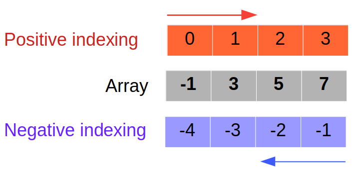
In contrast to Matlab, the indices in lists and numpy arrays in Python start from 0. Therefore, for an array of size \(n\) (in any of its dimensions), the indices range from 0 to \(n-1\). These are called positive (forward) indexing.
In contrast, we can have negative (backward) indexing: -1 (corresponding to \(n-1\)), -2 (corresponding to \(n-2\)), and so on. Note that -1 is the same as end in Matlab.
We can get the value of a specific element of an array by calling the array at the associated index.
1D Arrays:
print(x1)
print('Shape of x1:',x1.shape)
print('1st element of x1:',x1[0])
print('2nd element of x1:',x1[1])
print('Last element of x1:',x1[-1])
print('Second last element of x1:',x1[-2])
[-1.5  3.   5.   7.4]
Shape of x1: (4,)
1st element of x1: -1.5
2nd element of x1: 3.0
Last element of x1: 7.4
Second last element of x1: 5.0
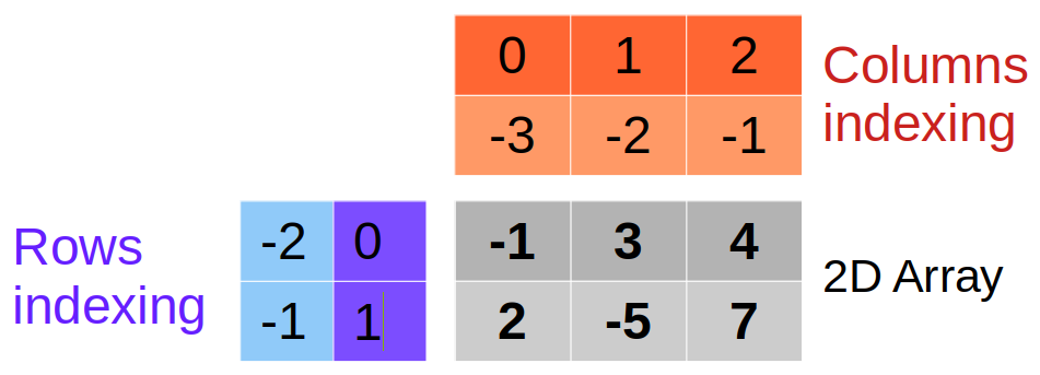
2D Arrays:
Combining the positive and negative indexing for the rows and columns, we have various ways of referring to the same element in the multidimensional arrays.
print(A1)
print('Shape of A1:',A1.shape)
print('Element A1[0,2]=',A1[0,2])
print('Element A1[-2,2]=',A1[-2,2])
print('Element A1[-2,-1]=',A1[-2,-1])
print('Element A1[0,-1]=',A1[0,-1])
[[-1.  3.  4.]
 [ 2. -5.  7.]]
Shape of A1: (2, 3)
Element A1[0,2]= 4.0
Element A1[-2,2]= 4.0
Element A1[-2,-1]= 4.0
Element A1[0,-1]= 4.0
5.4.2. Slicing#
Sometimes we need slices of data stored in an array. The slicing is applied by selecting a subrange of indices in different dimensions of an array. In general, over a given dimension, slicing from index m to n-1 is applied through m:n.
if no
mis provided, it is taken to be 0.if no
nis provided, it is taken to be -1.
See the following examples.
1d Arrays:
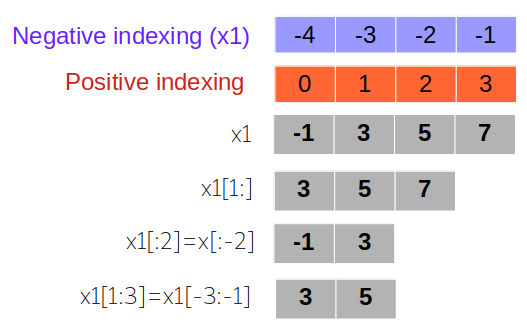
x1 = np.array([-1.5,3.,5.,7.4,5.7,9.8])
print('original array',x1)
original array [-1.5 3. 5. 7.4 5.7 9.8]
Select all elements starting from the 2nd one (index = 1):
print(x1[1:])
[3. 5. 7.4 5.7 9.8]
Select the first two elements:
print(x1[:2])
[-1.5 3. ]
Select all elements except the last two:
print(x1[:-2])
[-1.5 3. 5. 7.4]
Select the 2nd and 3rd elements:
print(x1[1:3])
[3. 5.]
Select the 3rd and 2nd last elements:
print(x1[-3:-1])
[7.4 5.7]
2D Arrays: We can follow the same rule along each of the two dimensions of a 2D array, selecting elements along rows and columns within some index range:
print(A2)
[[-1  3  4]
 [ 2 -5  7]
 [ 0  6  8]]
print(A2[1:,:-1])
print(A2[1:,:-1].shape)
[[ 2 -5]
 [ 0  6]]
(2, 2)
print(A2[1:2,:-2])
print(A2[1:2,:-2].shape)
[[2]]
(1, 1)
5.4.3. Axes#
Axes are properties particularly relevant to multidimensional numpy arrays. Many of the numpy built-in functions can be applied along a given axis of the array as well as along all axes (default).
A 1D numpy array has only one axis: 0.
A 2D numpy array has two axes: 0 and 1.
axis=0: Operates across rows (vertically).axis=1: Operates across columns (horizontally).
As a general rule for multidimensional arrays, axis=0 always refer to the operations along the outermost dimension. Thus, axis=1 refers to the second last dimension, and so on.
For instance, let’s consider the array A1 defined above:
print(A1)
[[-1.  3.  4.]
 [ 2. -5.  7.]]
If we want to find the sum over of all elements of this array, we simply use numpy.sum(A1):
print(np.sum(A1))
10.0
But, if we want to sum the rows together, we write
np.sum(A1, axis=0)
array([ 1., -2., 11.])
and to sum the columns:
np.sum(A1, axis=1)
array([6., 4.])
5.5. Some common arrays#
Here, we briefly review the syntax for creating a few common types of arrays.
5.5.1. Evenly-spaced numbers#
Assume that we want to create an array x where its elements are evenly spaced over a given range [a,b]. For this, we need to specify the size of x, i.e. the number of its elements. If this is denoted by n, then the space between each two successive elements of x is \(\Delta x = (b-a)/(n-1)\). Therefore, \(x\) is,
Although this can be done using a for loop (how?), we can instead use the built-in function numpy.linspace(start, stop, number), where
start: is the starting value = \(a\)end: is the end value = \(b\)number: is \(n\), the number of evenly-spaced values betweenstartandstopvalues.
Note that
All the above tree arguments are mandatory,
by default, the end value,
stop, is included in the generated array. To exclude it, we usenumpy.linspace(start, stop, number, endpoint=False). In this case, the above spacing \(\Delta x\) is changed to \((b-a)/n\).
For other options in this numpy function, see this link.
As a simple example, let’s generate 10 equi-spaced points over [1.2,5.6]:
x = np.linspace(1.2,5.6,10)
print(x)
[1.2        1.68888889 2.17777778 2.66666667 3.15555556 3.64444444
 4.13333333 4.62222222 5.11111111 5.6       ]
Let’s repeat the same example but excluding the end point:
x = np.linspace(1.2,5.6,10,endpoint=False)
print(x)
[1.2 1.64 2.08 2.52 2.96 3.4 3.84 4.28 4.72 5.16]
If we have an integer step size, we usually use the alternative function numpy.arange(start, stop, step), where,
start: is the starting value, (optional),stop: is the end value,step: step size, usually an integer (optional).
Note that only stop is the only mandatory input and,
startis by default 0,stepis by default 1.
To create an array of intergers from 0 to 9 (in total, 10 values), we write
x1 = np.arange(10)
print(x1)
[0 1 2 3 4 5 6 7 8 9]
If we want to start from a value else than 0:
x2 = np.arange(3,10)
print(x2)
[3 4 5 6 7 8 9]
We can use a step size other than 1:
x3 = np.arange(3,10,2)
print(x3)
[3 5 7 9]
What do you think happens if we use a real number as stop? Let’s test this:
x4 = np.arange(6.6)
print(x4)
[0. 1. 2. 3. 4. 5. 6.]
But if the start value is also a floating number, the output of arange is an array of floating values:
x5 = np.arange(2.1,6.6)
print(x5)
[2.1 3.1 4.1 5.1 6.1]
5.5.2. Identity matrix#
For an identity matrix, all elements are zero except the diagonal ones that are 1. An identity matrix of shape \(n\times n\) in numpy can be defined by I = numpy.identity(n). For instance, if \(n=4\), we have:
I = np.identity(4)
print(I)
[[1. 0. 0. 0.]
 [0. 1. 0. 0.]
 [0. 0. 1. 0.]
 [0. 0. 0. 1.]]
Exercise: Can you start from numpy.zero() and create the above identity matrix?
5.5.3. Random arrays#
Imagine we want to define an array with elements as random numbers. This can be done by classes in numpy.random that generate pseudo-random numbers. In particular,
numpy.random.rand(<array size>): returns an array of pseudo-random numbers with uniform distribution between 0 and 1.numpy.random.randn(<array size>): returns an array of pseudo-random numbers with standard Gaussian distribution (zero mean and variance 1).
u1 = np.random.rand(8)
g1 = np.random.randn(8)
print(u1)
print(g1)
[0.21749957 0.88005285 0.42455064 0.84364609 0.85066878 0.60211944
 0.78339773 0.88264178]
[ 0.27983129 -0.158244   -1.23871531 -1.19552706  0.80282082  1.02992682
  2.13679499 -0.14227631]
u2 = np.random.rand(3,2)
g2 = np.random.randn(3,2)
print(u2)
print(g2)
[[0.0475783  0.30838428]
 [0.27370091 0.33707851]
 [0.88509015 0.50889552]]
[[-0.34214199  0.43070078]
 [ 0.43300397  0.7600108 ]
 [-0.62573671  0.91001415]]
5.5.4. Diagonal elements/arrays#
You can extract the diagonal elements of a square matrix using numpy.diag().
print(np.diag(u2))
print(np.diag(g2))
[0.0475783  0.33707851]
[-0.34214199  0.7600108 ]
Moreover, numpy.diag() can be used to create a square matrix from a given 1D array. The elements of the 1D array will be the diagonal elements of the resulting matrix. The non-diagonal elements of the resulting will be 0.
d1 = np.array([1.2,5.6,2.4])

D1 = np.diag(d1)

print(D1)
[[1.2 0.  0. ]
 [0.  5.6 0. ]
 [0.  0.  2.4]]
5.5.5. Triangular matrices#
We can use numpy.tril(A) and numpy.triu(A) to respectively create a lower- and upper-triangular matrix from a given matrix A.
Lower-triangular matrix: All elements above the main diagonal are zero.
Upper-triangular matrix: All elements below the main diagonal are zero.
Consider the 2D array A2 defined above:
print(A2)
[[-1  3  4]
 [ 2 -5  7]
 [ 0  6  8]]
Its lower-triangular part is given by:
A2l = np.tril(A2)

print(A2l)
[[-1  0  0]
 [ 2 -5  0]
 [ 0  6  8]]
and its upper-triangular part by
A2u = np.triu(A2)

print(A2u)
[[-1  3  4]
 [ 0 -5  7]
 [ 0  0  8]]
5.6. Convert a list to a numpy array#
If we have a list of numbers, we can convert it to a numpy array of a desired shape. The conversion of a list to a numpy array is achieved through command asarray:
l = [1,2,6,-8,3,0]   # a list

la = np.asarray(l)   #conversion to numpy array

print('list:',l)
print('array:',la)
print('array shape:',la.shape)
list: [1, 2, 6, -8, 3, 0]
array: [ 1  2  6 -8  3  0]
array shape: (6,)
Similarly, multidimensional lists can be converted to numpy arrays:
l2 = [[1.,4.,-6.9],[-3.7, 8.1, - 0.2]]

l2a = np.asarray(l2)

print('list:',l2)
print('array:',l2a)
print('array shape:',l2a.shape)
list: [[1.0, 4.0, -6.9], [-3.7, 8.1, -0.2]]
array: [[ 1.   4.  -6.9]
 [-3.7  8.1 -0.2]]
array shape: (2, 3)
Note that contrary to the array, the list does NOT have a shape (among other attributes) and cannot be used with mathematical operations.
5.7. Reshape an array#
We can reshape a numpy array using numpy.reshape. Consider a 1D array x3 of size 6.
x3 = np.asarray([0,5,-7,8,10,12])
We can convert x3 to a 2D array of shape \(2 \times 3\) and \(3 \times 2\) as below:
x4 = np.reshape(x3,(2,3))

print(x4)
print(x4.shape)
[[ 0  5 -7]
 [ 8 10 12]]
(2, 3)
x5 = np.reshape(x3,(3,2))

print(x5)
print(x5.shape)
[[ 0  5]
 [-7  8]
 [10 12]]
(3, 2)
5.8. Concatenating arrays#
We can concatenate multiple arrays, provided their sizes match.
Let’s consider the following two arrays z1 and z2:
z1 = np.array([[2.2, -3.5]])
print(z1)
print('z1 shape:',z1.shape)
[[ 2.2 -3.5]]
z1 shape: (1, 2)
z2 = np.array([[1.4, 2.8], [-9.6,-7.3]])
print(z2)
print('z2 shape:',z2.shape)
[[ 1.4  2.8]
 [-9.6 -7.3]]
z2 shape: (2, 2)
We can concatenate z2 to z1 row-wise using numpy.concatenate (see this link):
z3 = np.concatenate((z1,z2),axis=0)
print(z3)
print('z3 shape:',z3.shape)
[[ 2.2 -3.5]
 [ 1.4  2.8]
 [-9.6 -7.3]]
z3 shape: (3, 2)
We can alternatively use numpy.vstack for vertically stacking the two arrays:
z4 = np.vstack((z1,z2))
print(z4)
print('z4 shape:',z4.shape)
[[ 2.2 -3.5]
 [ 1.4  2.8]
 [-9.6 -7.3]]
z4 shape: (3, 2)
For horizontally stacking arrays, we can use numpy.hstack. In this example, we can do this for the transpose of z1 stacked with z2:
z5 = np.hstack((z1.T,z2))
print(z5)
print('z5 shape:',z5.shape)
[[ 2.2  1.4  2.8]
 [-3.5 -9.6 -7.3]]
z5 shape: (2, 3)
5.9. Comparing arrays#
It is trivial that the value of corresponding elements in two arrays of similar shape can be compared to each other.
If we want to check if two arrays of similar shape are identical within a tolerance, i.e. all their elements are the same within a tolerance, we can use
numpy.allclose(array1, array2). The output of this is a Boolean value, i.e.TrueorFalse