14. Eigen decomposition

Saleh Rezaeiravesh, saleh.rezaeiravesh@manchester.ac.uk
Department of Mechanical and Aerospace Engineering, The University of Manchester, Manchester, UK

import numpy as np
import numpy.linalg as la

Overview: Eigenvalues and eigenvectors of matrices play a significant role in many theoretical problems and practical applications. The aim of this notebook is to show you how to use Python to perform eigen decomposition of matrices. The methods include the built-in functions from `numpy` and direct implementation of a few numerical algorithms.

14.1. Intended Learning Outcomes

After reading and running this notebook, the students should be able to:

• Use numpy built-in functions to compute eigenvalues and eigenvectors of matrices.

• Implement iterative algorithms to compute one or all eigenvalues of matrices.

14.2. Eigenvalues and eigenvectors of square matrices

Consider a square \(n\times n\) matrix \(\mathbf{A}\). Then the eigen decomposition of \(\mathbf{A}\) results in:

\[ \mathbf{A} \mathbf{x} = \lambda \mathbf{x} \]

where \(\lambda\) is an eigenvalue of \(\mathbf{A}\) and \(\mathbf{x}\) of size \(n\) is its corresponding eigenvector. The matrix \(\mathbf{A}\) has \(n\) eigenvalues and eigenvectors.

The above expression can be written as,

\[ (\mathbf{A} - \lambda \mathbf{I}) \mathbf{x} = \mathbf{0} \]

where \(\mathbf{I}\) is an identity matrix of the same size as \(\mathbf{A}\).

The eigenvalues are found from

\[ \det(\mathbf{A} - \lambda \mathbf{I}) = 0 \]

This equation leads to

\[ P(\lambda) = (-1)^n (\lambda^n+a_{n-1} \lambda^{n-1} + \cdots + a_1 \lambda + a_0) = 0 \]

where \(P(\lambda)\) is called the characteristic polynomial of \(\mathbf{A}\). Clearly, \(P(\lambda)\) is a polynomial of \(\lambda\) of order \(n\), hence it has \(n\) roots that are the eigenvalues of \(\mathbf{A}\). In practice, calculating thr roots of this polynomial is efficient only for low values of \(n\). Therefore, we require to use appropriate numerical algorithms to compute the eigenvalues of \(\mathbf{A}\).

Below, we show how to find the eigenvalues and eigenvectors of matrices in Python, using a numpy built-in function and also through direct implementation of a couple of algorithms.

14.3. numpy built-in function

For an \(n\times n\) matrix \(\mathbf{A}\), we have \(n\) eigenvalues and corresponding eigenvectors. All these \(n\) eigen pairs can be obtained at once using the numpy.linalg built-in function eigVals,eigVecs = eig(A).

Note that,

• eigVals is a 1D array of size \(n\) containing the eigenvalues of \(\mathbf{A}\),

• eigvecs is a \(n\times n\) matrix, the \(i\)-th column of which is the eigenvector corresponding to the \(i\)-th eigenvalue in eigVals.

Example: Let’s consider a \(3\times 3\) matrix:

A = np.array([[2.,8.,6.],[3.,4.,7.],[-2.,5.,-1.]])

The eigenvalues and eigenvectors of A are obtained as,

eigVals,eigVecs = la.eig(A)

Print the eigenvalues:

print('Eigenvalues:',eigVals)

Eigenvalues: [-5.03715425  0.58829246  9.44886179]

Print the array of eigenvectors (each column is an eigenvector of A):

print(eigVecs)

[[ 0.03520387 -0.8626677   0.7760559 ]
 [-0.61926264 -0.19710739  0.6137354 ]
 [ 0.78439434  0.46578227  0.14514166]]

Let’s check if the \(L_2\) norm of the eigenvectors is unity, i.e. \(\|\mathbf{x}\|_2=1\). Simply, we compute the norm of the columns of eigVecs:

for i in range(A.shape[0]):
    print('Norm of eigenvector %i = %g' %(i+1,la.norm(eigVecs[:,i],2)))

Norm of eigenvector 1 = 1
Norm of eigenvector 2 = 1
Norm of eigenvector 3 = 1

Example: The same numpy function can be used to find the complex eigenvalues of a matrix and its associated eigenvectors:

A = np.array([[3.,4.],[-5.,-5.]])

eigVals,eigVecs = la.eig(A) 

print(eigVals)

[-1.+2.j -1.-2.j]

print(eigVecs)

[[-0.59628479-0.2981424j -0.59628479+0.2981424j]
 [ 0.74535599+0.j         0.74535599-0.j       ]]

14.4. Implementation of Iterative algorithms

There are various algorithms to iteratively compute one or all eigenvalues of a matrix. In particular, we consider the following two methods:

• QR Method: returns all the eigenvalues of a real square matrix.

• Power Method: returns largest eigenvalue of a square matrix. Although it can be modified to compute other eigenvalues, but one at the time.

Below, we explain and implement these two algorithms.

14.4.1. QR method

The idea is to iteratively convert an input real square matrix \(\mathbf{A}\) into an upper-triangular matrix. Recall that the eigenvalues of an upper triangular matrix are the entries on its main diagonal.

In each iteration, a QR decomposition is needed, that is extensively discussed in the Matrix Decomposition notebook.

The following algorithm can be used to compute the eigenvalues of \(\mathbf{A}\) from its \(\mathbf{Q}\) (othogonal or normal matrix) and \(\mathbf{R}\) (upper triangular matrix) components.

Algorithm - QR method for finding eigenvalues of a real square matrix:

Input: An \(n\times n\) real matrix \(\mathbf{A}\)

1. Take \(\mathbf{A}_k = \mathbf{A}\)

2. While \(\mathbf{A}_k\) is not upper triangular:
   
   a. Compute the QR decomposition of \(\mathbf{A}_k = \mathbf{Q}_k \mathbf{R}_k\)
   
   b. Update \(\mathbf{A}_{k} = \mathbf{R}_k \mathbf{Q}_k\)

3. return \(\mathbf{A}_{k}\)

This algorithm is implemented in the following Python function where the QR decoomposition is performed by the built-in function numpy.linalg.qr().

def eig_QR(A):
    """
    Finding eigenvalues of a square real matrix A using the QR method
    """
    while not np.allclose(A, np.triu(A), atol=1e-06): #while A is not upper triangularized

        Q, R = la.qr(A)   #QR decomposition
        A = R @ Q         #update A
        
    return A

In the above implementation, we have used numpy.allclose(Atmp, numpy.triu(Atmp)) to check if all elements of Atmp and its upper triangular form are close enough. The latter means, the entries of the two arrays do not need to be exactly the same. The value of \(|a-b|\) with \(a\) and \(b\) being any corresponding elements in the two matrices should be below atol (absolute tolerance) for the matrices to be considered equal.

Let’s validate the results of this implementation against the built-in function numpy.linalg.eig():

Define an arbitrary real square matrix, and find its eigenvalues from the numpy function:

A = np.array([[2.,8.,6.],[3.,4.,7.],[-2.,5.,-1.]])

eigVals,eigVecs = la.eig(A) 

print('eig(A) - numpy:',eigVals)

eig(A) - numpy: [-5.03715425  0.58829246  9.44886179]

Now, call our function:

E = eig_QR(A)

The output should be an upper triangular matrix:

print(E)

[[ 9.44886197e+00 -3.56382406e+00  8.56571066e+00]
 [ 7.40930947e-07 -5.03715443e+00 -2.63206261e+00]
 [-2.11109557e-33  4.71184442e-26  5.88292464e-01]]

Since matrix \(\mathbf{E}\) is upper-triangular (the lower diaginal elements are apprximately zero - you can make atol smaller in numpy.allclose() to increase the accuracy), its diagonal elements are the eigenvalues of \(\mathbf{A}\).

print('eig(A), QR method:',np.diag(E))

eig(A), QR method: [ 9.44886197 -5.03715443  0.58829246]

These are very close to the eigenvalues computed by numpy.linalg.eig(A), confirming the validity of our implementation. Also the eigenvalues are sorted in a descending order in terms of magnitude.

14.4.2. Power method

The power method is an iterative method which can compute one eigenvalue at the time of a square matrix (the matrix is not necessarily real). Consider a \(n\times n\) matrix \(\mathbf{A}\). We can sort its eigenvalues in terms of their magnitude as,

\[ |\lambda_1| \leq |\lambda_2| \leq \cdots \leq |\lambda_n| \]

The following Power method algorithm computes \(\lambda_n\), i.e. the eigenvalue of \(\mathbf{A}\) with the largest magnitude and also its corresponding eigenvector:

Algorithm - Power method:

Inputs: An \(n\times n\) matrix \(\mathbf{A}\), a convergence tolerance \(\epsilon\)

1. Initial guess for the eigenvector corresponding to \(\lambda_n\): \(\mathbf{b}^{(0)}\) (a non-zero vector of size \(n\))

2. Initialize the error \(err\) (arbitrarily larger than \(\epsilon\))

3. While \(err\geq \epsilon\):

   a. Update the eigenvector:

   \[ \mathbf{b}^{(k+1)} = \frac{\mathbf{A} \mathbf{b}^{(k)}}{\|\mathbf{A}\mathbf{b}^{(k)}\|} \]

   b. Update the error: \(err= \|\mathbf{b}^{(k+1)}-\mathbf{b}^{(k)}\|\)

4. When converged, find the eigenvalue \(\lambda_n\):

   \[ \lambda_n^{(k+1)} = \frac{\langle \mathbf{A} \mathbf{b}^{(k+1)},\mathbf{b}^{(k+1)} \rangle}{\langle \mathbf{b}^{(k+1)},\mathbf{b}^{(k+1)}\rangle} \]

   where \(\langle \cdot , \cdot \rangle\) denotes an inner (dot) product.

def powerMethod(A,eps):
    """
    The power method to compute the eigenvalue of A with the largest magnitude
    
    Args:
      `A`: 2d numpy array, input matrix
      `eps`: float, convergence tolerance
      
    Returns
      `lam`: complex or float, largest-magnitude eigenvalue of A
      `b`: 1d numpy array, eigenvector associated with `lam`
      `errA`: list, collecting the error value after each iteration
    """
    
    n = A.shape[0]   #size of A    
    b = np.ones(n)   #initialize the eigenvector - an arbitrary non-zero vector   
    err = 10.*eps    #initial error value (arbitrarily larger than eps)
    errA = []        #initialize a list to collect the error after each iteration (optional)
    
    while err > eps:
       ab = A @ b           
       bnew = ab/la.norm(ab)  #compute the new eigenvector (normalized)
       err = la.norm(bnew-b)  #compute the error
       b = bnew               #update eigenvector b
       errA.append(err)       #collecting error in a list
    
    lam = np.dot(A @ b,b)/np.dot(b,b)    #eigenvalue of A corresponding to the eigenvector
    
    return lam,b,errA

Now, let’s apply this to find the eigenvalue with largest magnitude of a test matrix:

A = np.array([[2.,8.,6.],[3.,4.,7.],[-2.,5.,-1.]])


lam1, b1, errA1 = powerMethod(A, eps=1.e-6)

print('Largest mag. eigenvalue:',lam1)
print('Corresponding eigenvector:',b1)

Largest mag. eigenvalue: 9.448860839072196
Corresponding eigenvector: [0.77605584 0.61373553 0.14514144]

Our results can be validated against what we get from the built-in function numpy.linalg.eig(A):

eigVals,eigVecs = la.eig(A) 

print('eig(A) - numpy:',eigVals)

eig(A) - numpy: [-5.03715425  0.58829246  9.44886179]

print('eigenvectors:', eigVecs)

eigenvectors: [[ 0.03520387 -0.8626677   0.7760559 ]
 [-0.61926264 -0.19710739  0.6137354 ]
 [ 0.78439434  0.46578227  0.14514166]]

print(eigVecs@np.diag(eigVals)@la.inv(eigVecs))

[[ 2.  8.  6.]
 [ 3.  4.  7.]
 [-2.  5. -1.]]

Note that the column in eigVecs corresponding to the eigenvalue with the largest magnitude should be compared to our results.

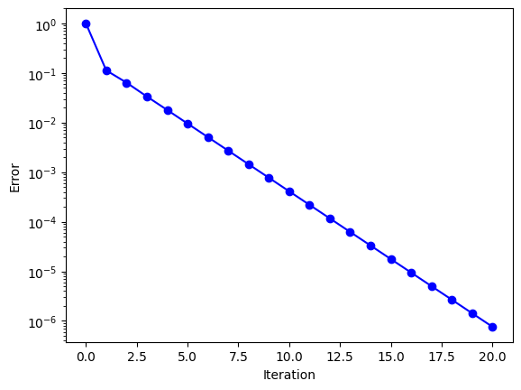
Finally, plotting the error in the Power method’s iterations shows the fast convergence of the algorithm for this particular example. Note that, the rate of onvergence of this algorithm is proportional to \(|\lambda_n|/|\lambda_{n-1}|\), the ratio of the largest to the second largest eigenvalue mangintude of \(\mathbf{A}\).

import matplotlib.pyplot as plt

plt.semilogy(np.arange(len(errA1)),errA1,'-ob')
plt.xlabel("Iteration")
plt.ylabel("Error")
plt.show()

14.4.2.1. Modifications of the power method

The Power method can also be used to find other eigen pairs of \(\mathbf{A}\). For instance, if the eigenvalue of \(\mathbf{A}\) with the smallest magnitude is needed, then we should find the eigenvalue with largest value of \(\mathbf{A}^{-1}\). Because, if \(\lambda\) is an eigenvalue of \(\mathbf{A}\), then \(1/\lambda\) is an eigenvalue of \(\mathbf{A}^{-1}\). The eigenvector corresponding to these eigenvalues is the same.

Example: For the following \(\mathbf{A}\), we apply the Power method to \(\mathbf{A}^{-1}\). This should return the eigenvalue of \(\mathbf{A}\) with smallest magnitude. However, to account for the negative sign,

A = np.array([[2.,8.,6.],[3.,4.,7.],[-2.,5.,-1.]])

Ainv = la.inv(A)  #A^{-1}

lam2, b2, errA2 = powerMethod(Ainv, eps=1.e-6)

We should reciprocate the computed eigenvalue to get the eigenvalue of \(\mathbf{A}\) with smallest magnitude.

print('Smallest magnitude eigenvalue of A:',1./lam2)

Smallest magnitude eigenvalue of A: 0.588292425883621