19. Interpolation and Function Approximation

Kristaps Stolarovs, Milan Mihajlovic and Aditya Mishra
kristaps.stolarovs@manchester.ac.uk
milan.mihajlovic@manchester.ac.uk
Department of Mechanical and Aerospace Engineering, The University of Manchester, Manchester, UK

import numpy as np
import matplotlib.pyplot as plt
import math
from sympy import symbols, expand, simplify, lambdify

Overview: Interpolation and function approximation are essential techniques in numerical analysis. Given a set of data points, interpolation methods construct functions that pass exactly through these points, while approximation methods build functions that represent the overall behavior of the data, typically minimising some error measure. This notebook explores several numerical approaches including Lagrange, Hermite, and Newton's interpolation methods, as well as discrete least squares approximation. We'll implement these techniques in Python and examine their mathematical foundations, computational characteristics, and practical applications.

19.1. Intended Learning Outcomes

After reading and running this notebook, the students should be able to:

• Implement Lagrange Interpolation to construct polynomials that pass through a given set of data points

• Apply Hermite Interpolation when both function values and derivatives are known

• Utilize Newton’s Interpolation with Divided Differences for sequential data fitting

• Employ Newton’s Finite Difference Interpolation Formulas for evenly spaced data

• Construct approximating functions using Discrete Least Squares methods to minimize error

19.2. Lagrange Interpolation

In general, interpolation involves creating a function \(y = f(x)\) for which a given set of points \({(x_i, y_i)}, i = 1, \cdots, n + 1\) satisfy \(y_i = f(x_i)\)

The discrete points may come from measurements or be values of some more complex function that we want to approximate.

Lagrange interpolation describes the process of finding a Lagrange interpolating polynomial, a unique polynomial of the lowest degree that interpolates a given set of data.

19.2.1. Theory

In Lagrange interpolation, a function \(f(x)\) given by its values \((x_i, y_i), i = 1, \ldots, n + 1\) is interpolated by an \(n\)-th order polynomial:

\[ P_n(x) = a_nx^n + a_{n-1}x^{n-1} + \cdots + a_1x + a_0 \]

Given \(n + 1\) distinct points \((x_0, y_0), (x_1, y_1), \cdots, (x_n, y_n)\), the Lagrange interpolating polynomial \(L(x)\) of degree at most \(n\) is:

\[ L(x) = \sum^n_{i=0} y_i \ell_i(x) \]

where \(\ell_i(x)\) are the Lagrange basis polynomials:

\[ \ell_i(x) = \prod_{j = 0,j \neq i}^n \frac{x - x_j}{x_i - x_j} \]

Each basis polynomial has the property that \(\ell_i(x_j) = 1\) if \(i = j\) and \(\ell_i(x_j) = 0\) if \(i \neq j\)

19.2.2. Example

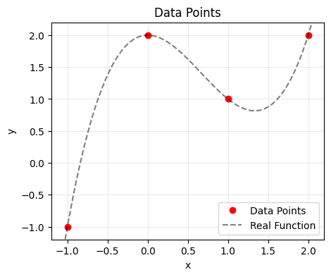
Let’s start with the following cubic function:

\[\begin{split} \begin{align} f(x) &= x^3 - 2x^2 + 2 \\ f'(x) &= 3x^2 - 4x \end{align} \end{split}\]

Utilising the following data-points:

\(x\)	\(y\)
-1	-1
0	2
1	1
2	2

# Main cubic function dataset
x = np.array([-1, 0, 1, 2])
xi = np.linspace(-1.5, 2.5, 100)

# Function and its derivative
def f1(x):
    return x**3 - 2*x**2 + 2
def df1(x):
    return 3*x**2 - 4*x

# Note: You can use Lambda functions for this.
# Lambda functions are small anonymous functions that are created with the lambda keyword.
# Lambda functions can have any number of arguments but only one expression. They are beyond the scope of this course.
# Example: f1 = lambda x: x**3 - 2*x**2 + 2
#          df1 = lambda x: 3*x**2 - 4*x

# Plot data points
plt.figure(figsize=(5, 4))
plt.grid(True, alpha=0.25)
plt.xlabel('x')
plt.ylabel('y')
plt.title('Data Points')

plt.plot(x, f1(x), 'ro', label='Data Points')
plt.plot(xi, f1(xi), 'k--', label='Real Function', alpha=0.5)

plt.xlim(-1.2, 2.2)
plt.ylim(-1.2, 2.2)

plt.legend()
plt.show()

We will now construct the Lagrange interpolation algorithm like so:

---

Input arrays \(\mathbf{X}\) and \(\mathbf{Y}\) of \(n\) data points, and point \(x_i\) to evaluate
Output interpolated value \(y_i\) at point \(x_i\)

\(y_i \leftarrow 0\)

for \(i \leftarrow 0\) to \(n-1\) do
\(\quad L_i \leftarrow 1\)
\(\quad\) for \(j \leftarrow 0\) to \(n-1\) do
\(\quad\quad\) if \(i \neq j\) then
\(\quad\quad\quad L_i \leftarrow L_i \times \frac{x_i - \mathbf{X}[j]}{\mathbf{X}[i] - \mathbf{X}[j]}\)
\(\quad y_i \leftarrow y_i + L_i \times \mathbf{Y}[i]\)

return \(y_i\)

---

def lagrange_interpolation(x, y, xi):
    n = len(x)  # Number of data points
    yi = 0      # Interpolated value at xi
    
    for i in range(n):
        
        # Calculate the Lagrange basis polynomial for point i
        L = 1
        for j in range(n):
            if i != j:
                L *= (xi - x[j]) / (x[i] - x[j])
                
        # Add the contribution of this basis polynomial
        yi += L * y[i]
    return yi

We can then give our data points to the algorithm, and it will obtain a lagrange interpolating polynomial:

# Interpolate
yi = [lagrange_interpolation(x, f1(x), xj) for xj in xi]

# Plot
plt.figure(figsize=(5, 4))
plt.scatter(x, f1(x), color='red', label='Data Points')
plt.plot(xi, yi, 'b-', label='Lagrange Polynomial')
plt.plot(xi, f1(xi), 'k--', label='Real Function', alpha=0.5)
plt.legend()
plt.xlabel('x')
plt.ylabel('y')
plt.title('Lagrange Interpolation, cubic function')
plt.grid(True, alpha=0.25)

plt.xlim(-1.2, 2.2)
plt.ylim(-1.2, 2.2)
plt.show()

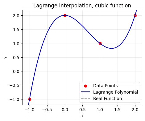
For our example data points, the Lagrange interpolation polynomial can be expressed as:

\[P(x) = ax^3 + bx^2 + cx + d\]

We can determine the coefficients by expanding the Lagrange formula using sympy:

# Define symbolic variable
x_sym = symbols('x')
y = f1(x)

# Calculate the symbolic Lagrange polynomial
L_sym = 0
for i in range(len(x)):
    basis = 1
    for j in range(len(x)):
        if i != j:
            basis *= (x_sym - x[j])/(x[i] - x[j])
    L_sym += y[i] * basis

# Expand and simplify
polynomial = expand(L_sym)
print("Lagrange polynomial:", polynomial)

Lagrange polynomial: x**3 - 2*x**2 + 2

The Lagrange polynomial recovered is:

\[ \begin{align} x^3 - 2x^2 + 2 \end{align} \]

Which, you will note, exactly matches the original function.

19.2.3. Challenging function

Let’s explore a case in which Lagrange interpolation may begin to struggle. Take this function:

\[ f(x) = \sin(2x) \times e^{-0.1x^2} \]

def f2(x):
    return np.sin(2*x) * np.exp(-0.1*x**2)
def df2(x):
    return 2*np.cos(2*x)*np.exp(-0.1*x**2) - 0.2*x*np.sin(2*x)*np.exp(-0.1*x**2)

# Interpolate
yi = [lagrange_interpolation(x, f2(x), xj) for xj in xi]

# Plot
plt.figure(figsize=(5, 4))
plt.scatter(x, f2(x), color='red', label='Data Points')
plt.plot(xi, yi, 'b-', label='Lagrange Polynomial')
plt.plot(xi, f2(xi), 'k--', label='Real Function', alpha=0.5)
plt.legend()
plt.xlabel('x')
plt.ylabel('y')
plt.title('Lagrange Interpolation, sinusoidal function')
plt.grid(True, alpha=0.25)

plt.xlim(-1.2, 2.2)
plt.ylim(-1.8, 1.2)
plt.show()

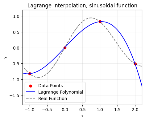
We can see that the Lagrange polynomial starts to struggle with accurately representing this more complex sinusoidal function. The interpolation passes through all the data points as expected, but significantly deviates from the true function between these points. This is particularly noticeable around x=0.75, where the Lagrange polynomial underestimates the peak of the function.

Of course the conclusion in this case is to use more / different sample points, but let us imagine a scenario where this is not possible. In this case, we can turn to Hermite interpolation.

19.3. Hermite Interpolation

Hermite interpolation extends the idea of Lagrange interpolation by also matching the derivatives at the interpolation points. In the case of Lagrange interpolation, we only knew the values of a function \(f(x)\) at interpolation points (knots) \(x_i\), \(i = 1, \ldots, m+1\). Hermite interpolation generalizes this by also incorporating derivative information at these knots.

19.3.1. Theory

At each point \(x_i\), we know not just the function value \(f(x_i)\), but also its derivatives \(f'(x_i)\), \(f''(x_i)\), etc. Therefore, we know the following values:

\[ f(x_i), f'(x_i), f''(x_i), \ldots, f^{(k_i-1)}(x_i), \quad i = 1,2,\ldots,m+1 \]

The number \(k_i\) is called the multiplicity of the knot \(x_i\). The total number of degrees of freedom (and the resulting polynomial degree plus one) is:

\[ n + 1 = k_1 + k_2 + \cdots + k_{m+1} \]

The Hermite interpolation polynomial \(H_n(x) = a_n x^n + \cdots + a_1 x + a_0\) must satisfy:

\[ H_n^{(j)}(x_i) = f^{(j)}(x_i), \quad i = 1,\ldots,m+1; \quad j = 0,1,\ldots,k_i-1 \]

This ensures the polynomial matches not just the function values but also all specified derivatives at each knot.

19.3.1.1. Simple case

For the special case where we know only function values and first derivatives (\(k_i = 2\) for all \(i\)), we can represent the Hermite polynomial as:

\[ H_n(x) = P_m(x) + (x-x_1)(x-x_2)\cdots(x-x_{m+1})H_k(x) \]

where \(P_m(x)\) is the Lagrange polynomial obtained only from function values, and \(H_k(x)\) is determined from the derivative information.

19.3.2. Implementation

For Hermite interpolation, we could directly solve for the polynomial coefficients, but there’s a more elegant approach using Newton’s divided differences:

---

Input arrays \(\mathbf{X}\) and \(\mathbf{Y}\) of \(m+1\) data points, array \(\mathbf{DY}\) of derivatives, and point \(x_i\) to evaluate
Output interpolated value \(y_i\) at point \(x_i\)

\(n \leftarrow m+1\) (number of knots)
Create array \(\mathbf{Z}\) of size \(2n\) for points with multiplicities
Create table \(\mathbf{Q}\) of size \(2n \times 2n\) for divided differences

for \(i \leftarrow 0\) to \(n-1\) do
\(\quad \mathbf{Z}[2i] \leftarrow \mathbf{X}[i]\), \(\mathbf{Z}[2i+1] \leftarrow \mathbf{X}[i]\) \(\quad \mathbf{Q}[2i, 0] \leftarrow \mathbf{Y}[i]\), \(\mathbf{Q}[2i+1, 0] \leftarrow \mathbf{Y}[i]\) \(\quad \mathbf{Q}[2i+1, 1] \leftarrow \mathbf{DY}[i]\) \(\quad\) if \(i \neq 0\) then
\(\quad\quad \mathbf{Q}[2i, 1] \leftarrow \frac{\mathbf{Q}[2i, 0] - \mathbf{Q}[2i-1, 0]}{\mathbf{Z}[2i] - \mathbf{Z}[2i-1]}\)

for \(i \leftarrow 2\) to \(2n-1\) do
\(\quad\) for \(j \leftarrow 2\) to \(i\) do
\(\quad\quad \mathbf{Q}[i, j] \leftarrow \frac{\mathbf{Q}[i, j-1] - \mathbf{Q}[i-1, j-1]}{\mathbf{Z}[i] - \mathbf{Z}[i-j]}\)

\(y_i \leftarrow \mathbf{Q}[0, 0]\)
for \(i \leftarrow 1\) to \(2n-1\) do
\(\quad term \leftarrow \mathbf{Q}[i, i]\)
\(\quad\) for \(j \leftarrow 0\) to \(i-1\) do
\(\quad\quad term \leftarrow term \times (x_i - \mathbf{Z}[j])\)
\(\quad y_i \leftarrow y_i + term\)

return \(y_i\)

---

This is a bare-bones implementation, you can also use various Python and numPy tools to make this easier. Please refer to the lecture notes for examples.

# Hermite Interpolation Implementation
def hermite_interpolation(x, y, dy, xi):
    n = len(x)                  # Number of data points
    z = np.zeros(2*n)           # Duplicate x values
    Q = np.zeros((2*n, 2*n))    # Divided differences table
    
    # Initialize the divided differences table
    for i in range(n):
        z[2*i] = z[2*i+1] = x[i]        # Duplicate x values
        Q[2*i, 0] = Q[2*i+1, 0] = y[i]  # Function values
        Q[2*i+1, 1] = dy[i]             # Derivative values
        if i != 0:
            Q[2*i, 1] = (Q[2*i, 0] - Q[2*i-1, 0]) / (z[2*i] - z[2*i-1])
    
    # Calculate the divided differences
    for i in range(2, 2*n):
        for j in range(2, i+1):
            Q[i, j] = (Q[i, j-1] - Q[i-1, j-1]) / (z[i] - z[i-j])
    
    # Evaluate the polynomial at xi
    yi = Q[0, 0]
    for i in range(1, 2*n):
        term = Q[i, i]
        for j in range(i):
            term *= (xi - z[j])
        yi += term
    
    return yi

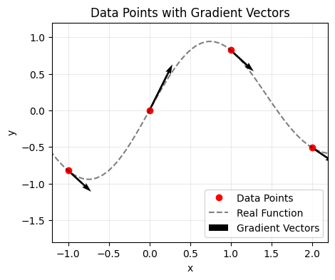
19.3.3. Example

For simplicity, our implementation will focus on the case where we know function values and first derivatives at each point (\(k_i = 2\) for all \(i\)).

Let’s use the same function as before, this time incorporating gradient information:

\[\begin{split} \begin{align} f(x) &= \sin(2x) \times e^{-0.1x^2} \\ f'(x) &= 2 \cos(2x) \times e^{-0.1x^2} - 0.2x \sin(2x) \times e^{-0.1x^2} \end{align} \end{split}\]

Effectively, this is what the algorithm now sees:

# Plot data points
plt.figure(figsize=(5, 4))
plt.grid(True, alpha=0.25)
plt.xlabel('x')
plt.ylabel('y')
plt.title('Data Points with Gradient Vectors')

plt.plot(x, f2(x), 'ro', label='Data Points')
plt.plot(xi, f2(xi), 'k--', label='Real Function', alpha=0.5)
plt.quiver(x, f2(x), np.ones(len(x)), df2(x), scale=12, color='k', label='Gradient Vectors', width=0.007)

plt.xlim(-1.2, 2.2)
plt.ylim(-1.8, 1.2)
plt.legend(loc='lower right')
plt.show()

# Interpolate
yi_lagrange = [lagrange_interpolation(x, f2(x), xj) for xj in xi]
yi_hermite = [hermite_interpolation(x, f2(x), df2(x), xj) for xj in xi]

# Plot
plt.figure(figsize=(5, 4))
plt.scatter(x, f2(x), color='red', label='Data Points')
plt.plot(xi, yi_lagrange, 'b-', label='Lagrange Polynomial')
plt.plot(xi, yi_hermite, 'g-', label='Hermite Polynomial')
plt.plot(xi, f2(xi), 'k--', label='Real Function', alpha=0.5)
plt.legend()
plt.xlabel('x')
plt.ylabel('y')
plt.title("Hermitian Interpolation, sinusoidal function")
plt.grid(True, alpha=0.25)

plt.xlim(-1.2, 2.2)
plt.ylim(-1.8, 1.2)
plt.show()

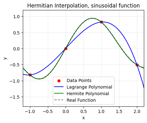
We can see that the Hermite polynomial is much more successful at capturing the real function thanks to the inclusion of the derivative information.

19.4. Newton’s Interpolation with Divided Differences

Newton’s divided differences interpolation provides a flexible and computationally efficient way to construct interpolation polynomials. Unlike the Lagrange form, Newton’s form makes it easy to add new interpolation points without recalculating the entire polynomial.

19.4.1. Theory

Given a set of points \((x_0, f(x_0)), (x_1, f(x_1)), \ldots, (x_n, f(x_n))\), Newton’s method uses divided differences to construct the interpolation polynomial.

The divided difference of the first order for the function \(f(x)\) at the points \(x_0\) and \(x_1\) is defined as:

\[ f[x_0, x_1] = \frac{f(x_1) - f(x_0)}{x_1 - x_0} \]

The divided difference of order \(k\) is defined recursively by:

\[ f[x_0, x_1, \ldots, x_k] = \frac{f[x_1, x_2, \ldots, x_k] - f[x_0, x_1, \ldots, x_{k-1}]}{x_k - x_0} \]

with the base case \(f[x] = f(x)\).

An alternative formula for the divided difference of order \(k\) is:

\[ f[x_0, x_1, \ldots, x_k] = \sum_{i=0}^{k} \frac{f(x_i)}{\omega'(x_i)} \]

where \(\omega(x) = (x - x_0)(x - x_1) \cdots (x - x_k)\) and \(\omega'(x_i)\) is the derivative of \(\omega(x)\) evaluated at \(x_i\).

19.4.2. Newton’s Interpolation Polynomial

Using divided differences, Newton’s interpolation polynomial for a dataset \((x_k, f(x_k))\), \(k = 0,1,\ldots,n\) is:

\[ P_n(x) = f(x_0) + (x - x_0)f[x_0, x_1] + (x - x_0)(x - x_1)f[x_0, x_1, x_2] + \ldots + (x - x_0)(x - x_1)\cdots(x - x_{n-1})f[x_0, x_1, \ldots, x_n] \]

This can be written more compactly as:

\[ P_n(x) = f(x_0) + \sum_{k=1}^{n} \left( f[x_0, x_1, \ldots, x_k] \prod_{i=0}^{k-1} (x - x_i) \right) \]

Since the algebraic interpolation polynomial is unique for a given set of points, Newton’s and Lagrange’s interpolation polynomials are equivalent, though they have different forms.

19.4.3. Implementation

The standard Newton’s divided differences algorithm is very similar to the earlier implementation of Hermite interpolation that we looked at earlier:

---

Input arrays \(\mathbf{x}\) and \(\mathbf{y}\) of \(n\) data points, and point \(x\) to evaluate
Output interpolated value \(p\) at point \(x\)

function divided_diff(\(\mathbf{x}\), \(\mathbf{y}\)):
\(\quad n \leftarrow \text{len}(y)\)
\(\quad \text{coef} \leftarrow \text{zeros}[n, n]\)
\(\quad \text{coef}[:,0] \leftarrow \mathbf{y}\)
\(\quad\) for \(j \leftarrow 1\) to \(n-1\) do
\(\quad\quad\) for \(i \leftarrow 0\) to \(n-j-1\) do
\(\quad\quad\quad \text{coef}[i][j] \leftarrow \frac{\text{coef}[i+1][j-1] - \text{coef}[i][j-1]}{\mathbf{x}[i+j] - \mathbf{x}[i]}\)
\(\quad\) return \(\text{coef}[0, :]\)

function newton_poly(\(\text{coef}\), \(\mathbf{x\_data}\), \(x\)):
\(\quad n \leftarrow \text{len(coef)}\)
\(\quad p \leftarrow \text{coef}[0]\)
\(\quad\) for \(k \leftarrow 1\) to \(n-1\) do
\(\quad\quad \text{term} \leftarrow \text{coef}[k]\)
\(\quad\quad\) for \(j \leftarrow 0\) to \(k-1\) do
\(\quad\quad\quad \text{term} \leftarrow \text{term} \times (x - \mathbf{x\_data}[j])\)
\(\quad\quad p \leftarrow p + \text{term}\)
\(\quad\) return \(p\)

---

The algorithm first calculates the divided difference coefficients, then evaluates the polynomial at the desired point.

# Newton's Divided Differences Interpolation Implementation
def divided_diff(x, y):
    n = len(y)
    coef = np.zeros([n, n])
    coef[:,0] = y
    for j in range(1,n):
        for i in range(n-j):
            coef[i][j] = (coef[i+1][j-1] - coef[i][j-1]) / (x[i+j] - x[i])
    return coef[0, :]

def newton_poly(coef, x_data, x):
    n = len(coef)
    p = coef[0]
    for k in range(1, n):
        term = coef[k]
        for j in range(k):
            term = term * (x - x_data[j])
        p = p + term
    return p

19.4.4. Example

Let’s apply Newton’s divided differences to the cubic function we used earlier:

\[ f(x) = x^3 - 2x^2 + 2\]

# Interpolate (and calculate the divided differences)
coef = divided_diff(x, f1(x))
yi_newton = [newton_poly(coef, x, xj) for xj in xi]

# Plot
plt.figure(figsize=(5, 4))
plt.scatter(x, f1(x), color='red', label='Data Points')
plt.plot(xi, yi_newton, 'c-', label='Newton Polynomial')
plt.plot(xi, f1(xi), 'k--', label='Real Function', alpha=0.5)
plt.legend()
plt.xlabel('x')
plt.ylabel('y')
plt.title('Newton Divided Differences, cubic function')
plt.grid(True, alpha=0.25)

plt.xlim(-1.2, 2.2)
plt.ylim(-1.2, 2.2)
plt.show()

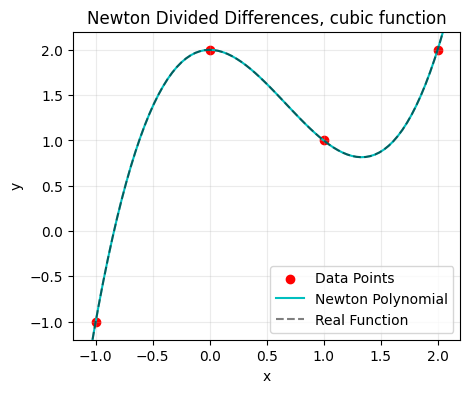
While Newton’s and Lagrange’s methods produce mathematically identical polynomials for the same dataset, Newton’s approach offers practical advantages (non-exhaustive list):

1. Incremental computation: Newton’s form allows adding new points without recalculating the entire polynomial

2. Computational efficiency: Often requires fewer operations when evaluating at multiple points

3. Numerical stability Can be more stable for certain datasets

There are many other factors to consider when deciding between interpolation schemes, but this hopefully gives an idea to the differences between seemingly similar methods.

19.5. Discrete Least Squares Approximation

Unlike interpolation methods which create functions that pass exactly through all data points, approximation methods aim to find a function that represents the overall trend of the data, possibly smoothing out noise or simplifying complex patterns.

19.5.1. Theory

We consider a function \(f(x): [a, b] \rightarrow \mathbb{R}\) given by pairs of values \((x_i, f_i)\), \(i = 0, \ldots, m\), where \(f_i = f(x_i)\). We want to approximate \(f(x)\) by:

\[ \phi(x) = a_0\phi_0(x) + a_1\phi_1(x) + \cdots + a_n\phi_n(x) \]

Note that, in general, \(m \neq n\). In previous sections (interpolation), we considered the simple case when \(m = n\) and \(\phi_i(x) = x^i\), resulting in a polynomial approximation:

\[ \phi(x) = a_0 + a_1x + \cdots + a_nx^n \]

In least squares approximation, we’re concerned with the overdetermined case where \(m > n\) (we have more data points than basis functions). This means we cannot find coefficients that make our approximation pass through all points exactly.

From the conditions \(f_i = \phi(x_i)\), we obtain the following overdetermined system of equations:

\[\begin{split} \begin{align} a_0\phi_0(x_0) + a_1\phi_1(x_0) + \cdots + a_n\phi_n(x_0) &= f_0\\ a_0\phi_0(x_1) + a_1\phi_1(x_1) + \cdots + a_n\phi_n(x_1) &= f_1\\ \vdots\\ a_0\phi_0(x_m) + a_1\phi_1(x_m) + \cdots + a_n\phi_n(x_m) &= f_m \end{align} \end{split}\]

Since this system is overdetermined, it generally doesn’t have an exact solution. Instead, we look for coefficients that minimise the overall error.

19.5.2. Error Minimisation

We define the error at each point as: $\( \delta_n = f(x) - \phi(x) \)$

And seek the solution which minimises the sum of squared errors, i.e., find \(a_0^*, a_1^*, \ldots, a_n^*\) such that: $\( \|\delta_n^*\|_2^2 = \min_{a_i} \|\delta_n\|_2^2 \)$

where: $\( \|\delta_n\|_2^2 = \sum_{j=0}^{m} \delta_n(x_j)^2 = \sum_{j=0}^{m} (f(x_j) - \phi(x_j))^2 \)$

19.5.3. Matrix Formulation

Using matrix notation, we can represent our problem more compactly:

\[\begin{split} \Phi = \begin{pmatrix} \phi_0(x_0) & \phi_1(x_0) & \cdots & \phi_n(x_0) \\ \phi_0(x_1) & \phi_1(x_1) & \cdots & \phi_n(x_1) \\ \vdots & \vdots & \ddots & \vdots \\ \phi_0(x_m) & \phi_1(x_m) & \cdots & \phi_n(x_m) \end{pmatrix}, \mathbf{f} = \begin{pmatrix} f_0 \\ f_1 \\ \vdots \\ f_m \end{pmatrix}, \mathbf{a} = \begin{pmatrix} a_0 \\ a_1 \\ \vdots \\ a_n \end{pmatrix} \end{split}\]

If we define \(\mathbf{v} = \mathbf{f} - \Phi\mathbf{a}\), then \(\|\delta_n\|_2^2 = \mathbf{v}^T\mathbf{v}\).

19.5.4. Normal Equations

Minimising \(\|\delta_n\|_2^2\) leads to a system of equations: $\( \Phi^T\mathbf{v} = \mathbf{0} \)$

which is equivalent to: $\( \Phi^T\Phi\mathbf{a} = \Phi^T\mathbf{f} \)$

These are called the normal equations. This system is obtained from the overdetermined system \(\Phi\mathbf{a} = \mathbf{f}\) by pre-multiplication with \(\Phi^T\).

19.5.5. Implementation

Let’s implement the discrete least squares method for polynomial approximation, where \(\phi_i(x) = x^i\):

def least_squares_approximation(x, y, n):
    m = len(x)
    
    # Build the Phi matrix
    Phi = np.zeros((m, n+1))
    for i in range(m):
        for j in range(n+1):
            Phi[i, j] = x[i]**j

    # Calculate normal equations: (Phi^T * Phi) * a = Phi^T * f
    PhiT_Phi = np.dot(Phi.T, Phi)
    PhiT_f = np.dot(Phi.T, y)
    
    c = np.linalg.solve(PhiT_Phi, PhiT_f)   # Solve the linear system
    
    return c

def eval_poly(c, x):
    
    # Evaluate the polynomial at x
    y = 0
    for i, coef in enumerate(c):
        y += coef * x**i
    return y

19.5.6. Example

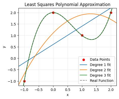
The method is able to relatively easily capture our original function:

\[ f(x) = x^3 - 2x^2 + 2\]

# Approximate the function with a polynomial
n = [1, 2, 3]   # Polynomial degrees, we know that the function is cubic
c = [least_squares_approximation(x, f1(x), degree) for degree in n]
yi_dls = [eval_poly(c[i], xi) for i in range(len(n))]

# Plot the results
plt.figure(figsize=(5, 4))
plt.grid(True, alpha=0.25)
plt.scatter(x, f1(x), color='red', label='Data Points')

for i, degree in enumerate(n):
        plt.plot(xi, yi_dls[i], label=f'Degree {degree} fit')

plt.plot(xi, f1(xi), 'k--', label='Real Function', alpha=0.5)

plt.legend()
plt.xlabel('x')
plt.ylabel('y')
plt.title('Least Squares Polynomial Approximation')
plt.grid(True, alpha=0.25)

plt.xlim(-1.2, 2.2)
plt.ylim(-1.2, 2.2)
plt.show()

19.5.7. Noisy Datasets

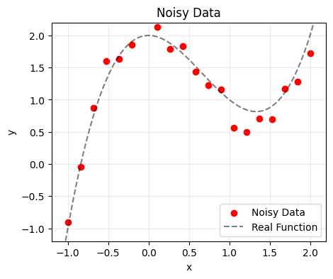
Discrete least squares approximation become particularly useful when we have noisy data:

# Noisy data
np.random.seed(42)
x_dls = np.linspace(-1, 2, 20)
yi_noise = f1(x_dls) + 0.2*np.random.randn(len(x_dls))

# Plot the noisy data
plt.figure(figsize=(5, 4))

plt.scatter(x_dls, yi_noise, color='red', label='Noisy Data')
plt.plot(xi, f1(xi), 'k--', label='Real Function', alpha=0.5)

plt.legend()
plt.xlabel('x')
plt.ylabel('y')
plt.title('Noisy Data')
plt.grid(True, alpha=0.25)

plt.xlim(-1.2, 2.2)
plt.ylim(-1.2, 2.2)
plt.show()

If we try to fit this using an interpolation method (such as Lagrange), we will have very questionable results:

# Lagrange interpolation
yi_lagrange = [lagrange_interpolation(x_dls, yi_noise, xj) for xj in xi]

# Plot
plt.figure(figsize=(5, 4))
plt.scatter(x_dls, yi_noise, color='red', label='Noisy Data')
plt.plot(xi, yi_lagrange, 'b-', label='Lagrange Polynomial')
plt.plot(xi, f1(xi), 'k--', label='Real Function', alpha=0.5)

plt.legend()
plt.xlabel('x')
plt.ylabel('y')
plt.title('Lagrange Interpolation, noisy data')
plt.grid(True, alpha=0.25)

plt.xlim(-1.2, 2.2)
plt.ylim(-1.2, 2.2)
plt.show()

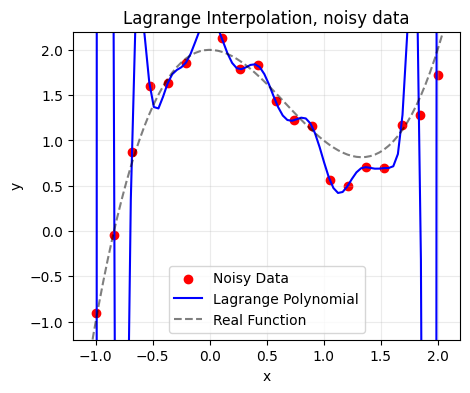
Which is when we turn to approximation. In this case, we will be evaluating a series of degrees and picking the degree with the smallest error.

# Evaluate the polynomial at x
n = [1, 2, 3]
c = [least_squares_approximation(x_dls, yi_noise, degree) for degree in n]
yi_dls = [eval_poly(c[i], xi) for i in range(len(n))]

# Plot the results
plt.figure(figsize=(5, 4))

plt.scatter(x_dls, yi_noise, color='red', label='Noisy Data Points')

for i, degree in enumerate(n):
    plt.plot(xi, yi_dls[i], label=f'Degree {degree} fit')

plt.plot(xi, f1(xi), 'k--', label='Real Function', alpha=0.5)

plt.legend()
plt.xlabel('x')
plt.ylabel('y')
plt.title('Least Squares Polynomial Approximation with Noise')
plt.grid(True, alpha=0.25)

plt.xlim(-1.2, 2.2)
plt.ylim(-1.2, 2.2)
plt.show()

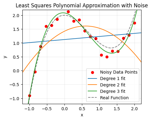
for degree in n:
    coeffs = least_squares_approximation(x_dls, yi_noise, degree)
    y_fit = eval_poly(coeffs, x_dls)
    sse = np.sum((yi_noise - y_fit)**2)
    print(f"Degree {degree}: Sum of squared errors = {sse:.6f}")

Degree 1: Sum of squared errors = 11.193967
Degree 2: Sum of squared errors = 8.302696
Degree 3: Sum of squared errors = 0.395576

It is important to note however that these approximation techniques are susceptible to overfitting. If we tried to use a degree of \(n = 20\), we would likely see a lower error, even though, due to our knwoledge of the underlying function, we know that the ideal solution is \(n = 3\). There are multiple approaches that can be used to combat this, but they are outside of the scope of the course.