17. Iterative methods for solving linear systems#
Saleh Rezaeiravesh, saleh.rezaeiravesh@manchester.ac.uk
Department of Mechanical and Aerospace Engineering, The University of Manchester, Manchester, UK
17.1. Intended Learning Outcomes#
After reading and running this notebook, the students should be able to:
Understand the algorithm of iterative methods for solving linear systems.
Develop Python functions/scripts for iterative solvers of linear systems using
numpyarrays and functions.
17.2. Import libraries#
In this notebook, we rely on the methods provided by numpy and numpy.linalg.
import numpy as np
import numpy.linalg as la
17.3. System of linear equations#
Consider the following system of linear equations,
where,
\(a_{ij}\): known coefficients, \(i,j=1,2,\cdots,n\),
\(b_i\): right-hand side values, \(i=1,2,\ldots,n\)
\(x_j\): unknown solutions, \(j=1,2,\ldots,n\).
We can rewrite this system in a matrix form:
where,
\(\mathbf{A}\) is an \(n\times n\) matrix (coefficient matrix),
\(\mathbf{x}\) is an \(n\times 1\) matrix (solution vector),
\(\mathbf{b}\) is an \(n\times 1\) matrix (right-hand-side (RHS) vector).
In the following sections, we demonstrate how to write Python functions to solve linear systems adopting different iterative methods. For the direct methods, refer to this notebook.
17.4. General formulation of iterative solvers#
In the iterative algorithms for solving the linear system (1), we start from and initial guess \(\mathbf{x}^{(0)}\) and then find the solution \(\mathbf{x}\) with a pre-defined accuracy through a finite number of iterations.
The general expression to update the iterative solution \(\mathbf{x}^{(k)}\) given the old (last iteration) solution \(\mathbf{x}^{(k-1)}\) is written as,
where \(n\times n\) matrices \(\mathbf{B}\) and \(\mathbf{C}\) are determined for a given \(\mathbf{A}\) based on different iteration methods, see below.
Starting from an initial guess \(\mathbf{x}^{(0)}\), equation (2) is used for updating the sequence \(\mathbf{x}^{(0)}, \mathbf{x}^{(1)}, \cdots, \mathbf{x}^{(k)}\), until at the \(m\)-th iteration, the magnitude of the residual vector \(r^{(m)}\) becomes less than a specified threshold \(\epsilon\) multiplied by the magnitude of the initial residual vector \(\|\mathbf{r}^{(0)}\|\), i.e. when,
where \(\mathbf{r}^{(k)} = \mathbf{A}\mathbf{x}^{(k)}-\mathbf{b}\) for \(k=1,2,\cdots\). Note that, we can use different types of norm to find the magnitude of the residual vector.
In practice, we need to check if the adopted iteration method is converging for the given problem. To this end, after \(\textbf{B}\) is computed, we should check if the following sufficient condition for convergence is satisfied:
This means, the absolute value (magnitude) of all eigenvalues of \(\mathbf{B}\) must be less than \(1\) to ensure the iterations will converge.
17.5. General algorithm for iterative solution of linear systems#
The main steps of iterative methods to solve linear systems are provided below:
Inputs: An \(n\times n\) matrix \(\mathbf{A}\) and a vector \(\mathbf{b}\) of size \(n\).
Based on the particular iterative method, find \(\mathbf{B}\) and \(\mathbf{C}\).
Choose \(\varepsilon\), the maximum error below which iterations stop.
Make an initial guess for the solution: \(\mathbf{x}^{(0)}\)
Calculate initial residual vector \(\mathbf{r}^{(0)}=\mathbf{A}\mathbf{x}^{(0)}-\mathbf{b}\).
While \(\|\mathbf{r}^{(k)}\| > \varepsilon \|\mathbf{r}^{(0)}\|\) (iteration loop)
a. Update the solution: \(\mathbf{x}^{(k)} = \mathbf{B}\mathbf{x}^{(k-1)} + \mathbf{C}\mathbf{b}\)
b. Calculate the residual of the new solution: \(\mathbf{r}^{(k)}=\mathbf{A}\mathbf{x}^{(k)}-\mathbf{b}\)
Below, we refine this algorithm for different iteration methods.
17.6. Simple iteration method#
Rewrite the linear system (1) as,
The simple iteration method:
Comparing this to the general expression (2), we have the following \(\mathbf{B}\) and \(\mathbf{C}\):
The following function implements the simple iteration method to solve (1). The inputs to the function are the coefficient matrix \(\mathbf{A}\), the right-hand-side (RHS) vector \(\mathbf{b}\), and the convergence tolerance \(\varepsilon\) (eps, a small positive value). The outputs of the functions are the converged solution for \(\mathbf{x}\) and the number of iterations to reach convergence.
Note that in the function, we check the magnitude of the eigenvalues of \(\mathbf{B}\). If the sufficient convergence condition holds true, the iterations are performed; otherwise, the function is terminated with an error.
def simpleIter(A,b,eps):
    """
    Simple iteration method to solve linear system A x = b

    Args:
       `A`: numpy array of shape n-by-n, coefficient matrix
       `b`: numpy array of size n, right-hand-side vector
       `eps`: float, convergence tolerance

    Returns:
       `x`: numpy array of size n, converged solution of the linear system
       `k`: int, number of iterations to reach convergence
    """
    n = len(b)   #system size

    xold = np.zeros(n)  #initial guess for x

    resid0 = la.norm(A @ xold - b)   #norm of the initial residual
    resid = resid0

    B = np.identity(n)-A    #create B = I-A

    #check if the sufficient condition for convergence holds
    eB, vB = la.eig(B)
    print("Eigenvalues of B:",eB)
    if np.max(abs(eB)) > 1:
       print("Eigenvalues of B:",eB)
       raise ValueError("Sufficient condition for convergence does not hold!")

    #iteration loop
    k=0         #iteration counter

    while resid > eps*resid0:
        x = B @ xold + b           #update x
        resid = la.norm(A @ x - b) #norm of the new residual
        xold = x
        k += 1

    return x,k
Example: Let’s apply the above function for a linear system, and validate its results with the direct inversion method.
A = np.array([[0.5,0.2,-0.1],[0.4,0.8,-0.6],[0.2,-0.3,0.7]])
b = np.array([3., -2.,4.])

xs, ks = simpleIter(A,b,eps=1.e-6)
Eigenvalues of B: [ 0.80990195 0.4 -0.20990195]
print('Number of iterations:', ks)
print('Converged solution for x:', xs)
print('Reference solution (direct inversion)', la.inv(A) @ b)
Number of iterations: 62
Converged solution for x: [ 8.69564421 -6.52171944  0.43479732]
Reference solution (direct inversion) [ 8.69565217 -6.52173913  0.43478261]
Clearly, the approximate solution \(\mathbf{x}\) is very close to the exact solution found from \(\mathbf{x}=\mathbf{A}^{-1}\mathbf{b}\). You can try to change the value of the tolerance \(\varepsilon\), eps, when calling simpleIter() function, and investigate its impact on the solution’s accuracy.
17.7. Jacobi iteration method#
In the linear system (1), the coefficient matrix \(\mathbf{A}\) can be decomposed as,
Using this decomposition, the Jacobi iteration method reads as:
Comparing this to the general expression (2), we have the following \(\mathbf{B}\) and \(\mathbf{C}\):
The following function implements the simple iteration method to solve (1). The inputs to the function are the coefficient matrix \(\mathbf{A}\), the right-hand-side (RHS) vector \(\mathbf{b}\), and the convergence tolerance \(\varepsilon\) (eps, a small positive value). The outputs of the functions are the converged solution for \(\mathbf{x}\), the number of iterations to reach convergence, and also the residA list of residual anorm at all iterations. The latter can be used to make a plot for the reduction of residuals as a result of the iterations.
Note that in the function, we check the magnitude of the eigenvalues of \(\mathbf{B}\). If the sufficient convergence condition holds true, the iterations are performed; otherwise, the function is terminated with an error.
def jacobiIter(A,b,eps):
    """
    Jacobi iteration method to solve linear system A x = b

    Args:
       `A`: numpy array of shape n-by-n, coefficient matrix
       `b`: numpy array of size n, right-hand-side vector
       `eps`: float, convergence tolerance

    Returns:
       `x`: numpy array of size n, converged solution of the linear system
       `k`: int, number of iterations to reach convergence
       `residA`: list, norm of the residual at different iterations
    """
    n = len(b)   #system size

    xold = np.zeros(n)  #initial guess for x

    resid0 = la.norm(A @ xold - b)   #norm of the initial residual
    resid = resid0

    #find B, C associated with the Jacobi method
    D = np.diag(np.diag(A))   #A square matrix with diagonal elements of A
    M = A - D                 #M = A-D
    B = - la.inv(D) @ M
    Cb = la.inv(D) @ b

    #check if the sufficient condition for convergence holds
    eB, vB = la.eig(B)
    if np.max(abs(eB)) > 1:
       print("Eigenvalues of B:",eB)
       raise ValueError("Sufficient condition for convergence does not hold!")

    #iteration loop
    k = 0                #iteration counter
    residA = [resid0]    #list to save the residual magnitude during the iterations

    while resid > eps*resid0:
        x = B @ xold + Cb           #update x
        resid = la.norm(A @ x - b) #norm of the new residual
        xold = x
        k += 1
        residA.append(resid)

    return x,k,residA
Example: We can apply the above function for solving any linear system (conditioned on the coefficient matrix being square), and validate the resulting solution against the solution from direct inversion of the linear system.
A = np.array([[4., 2., -1., 1.],[1., 4., -2., -1.],[-1, 2., 7., 1.],[2., -1., 2., 6.]])
b = np.array([4.6, -3.5, 8., 6.4])

xJ, kJ, rJ = jacobiIter(A,b,eps=1.e-6)
print('Number of iterations:', kJ)
print('Converged solution for x:', xJ)
print('Reference solution (direct inversion)', la.inv(A) @ b)
Number of iterations: 24
Converged solution for x: [ 1.9018304  -0.59470387  1.61364392 -0.20427428]
Reference solution (direct inversion) [ 1.90183299 -0.59470468  1.61364562 -0.20427699]
17.8. Gauss-Seidel iteration method#
To reduce the number of iterations, we can apply the Gauss-Seidel algorithm:
In the linear system (1), the coefficient matrix \(\mathbf{A}\) can be decomposed as,
where
Using the above decomposition, the Gauss-Seidel iteration method reads as:
Comparing this to the general expression (2), we have the following \(\mathbf{B}\) and \(\mathbf{C}\):
and
The following function implements the simple iteration method to solve (1). The inputs to the function are the coefficient matrix \(\mathbf{A}\), the right-hand-side (RHS) vector \(\mathbf{b}\), and the convergence tolerance \(\varepsilon\) (eps, a small positive value). The outputs of the functions are the converged solution for \(\mathbf{x}\), the number of iterations to reach convergence, and also the residA list of residual anorm at all iterations. The latter can be used to make a plot for the reduction of residuals as a result of the iterations.
Note that in the function, we check the magnitude of the eigenvalues of \(\mathbf{B}\). If the sufficient convergence condition holds true, the iterations are performed; otherwise, the function is terminated with an error.
def gaussSeidelIter(A,b,eps):
    """
    Gauss-Seidel iteration method to solve linear system A x = b

    Args:
       `A`: numpy array of shape n-by-n, coefficient matrix
       `b`: numpy array of size n, right-hand-side vector
       `eps`: float, convergence tolerance

    Returns:
       `x`: numpy array of size n, converged solution of the linear system
       `k`: int, number of iterations to reach convergence
       `residA`: list, norm of the residual at different iterations
    """
    n = len(b)   #system size

    xold = np.zeros(n)  #initial guess for x

    resid0 = la.norm(A @ xold - b)   #norm of the initial residual
    resid = resid0

    #find B, C associated with the Jacobi method
    D = np.diag(A)
    U = np.triu(A-np.diag(D))
    L = np.tril(A)
    B = -la.inv(L) @ U
    Cb = la.inv(L) @ b

    #check if the sufficient condition for convergence holds
    eB, vB = la.eig(B)
    if np.max(abs(eB)) > 1:
       print("Eigenvalues of B:",eB)
       raise ValueError("Sufficient condition for convergence does not hold!")

    #iteration loop
    k = 0                #iteration counter
    residA = [resid0]    #list to save the residual magnitude during the iterations

    while resid > eps*resid0:
        x = B @ xold + Cb           #update x
        resid = la.norm(A @ x - b) #norm of the new residual
        xold = x
        k += 1
        residA.append(resid)

    return x,k,residA
Example: We can apply the above function for solving any linear system (conditioned on the coefficient matrix being square), and validate the resulting solution against the solution from direct inversion of the linear system.
A = np.array([[4., 2., -1., 1.],[1., 4., -2., -1.],[-1, 2., 7., 1.],[2., -1., 2., 6.]])
b = np.array([4.6, -3.5, 8., 6.4])

xGS, kGS, rGS = gaussSeidelIter(A,b,eps=1.e-6)
print('Number of iterations:', kGS)
print('Converged solution for x:', xGS)
print('Reference solution (direct inversion)', la.inv(A) @ b)
Number of iterations: 10
Converged solution for x: [ 1.90182894 -0.59470396  1.61364402 -0.20427498]
Reference solution (direct inversion) [ 1.90183299 -0.59470468  1.61364562 -0.20427699]
17.9. SOR iteration method#
The Successive Over-relaxation (SOR) method is a modified version of the Gauss-Seidel method:
where \(\omega\) is the relaxation factor. Clearly for \(\omega=1\), the Gauss-Seidel iterations are recovered.
The following function implements the SOR method to solve linear systems. Here, there is an additional input parameter \(\omega\).
def SORIter(A,b,w,eps):
    """
    SOR method to solve linear system A x = b

    Args:
       `A`: numpy array of shape n-by-n, coefficient matrix
       `b`: numpy array of size n, right-hand-side vector
       `w`: float, relaxation factor
       `eps`: float, convergence tolerance

    Returns:
       `x`: numpy array of size n, converged solution of the linear system
       `k`: int, number of iterations to reach convergence
       `residA`: list, norm of the residual at different iterations
    """
    n = len(b)   #system size

    xold = np.zeros(n)  #initial guess for x

    resid0 = la.norm(A @ xold - b)   #norm of the initial residual
    resid = resid0

    #find B, C associated with the Jacobi method
    D = np.diag(np.diag(A))
    U = np.triu(A-D)
    L = np.tril(A)-D
    B = -la.inv(D+w*L) @ ((w-1.)*D+w*U)
    Cb = la.inv(D+w*L) @ (w*b)

    #check if the sufficient condition for convergence holds
    eB, vB = la.eig(B)
    if np.max(abs(eB)) > 1:
       print("Eigenvalues of B:",eB)
       raise ValueError("Sufficient condition for convergence does not hold!")

    #iteration loop
    k = 0                #iteration counter
    residA = [resid0]    #list to save the residual magnitude during the iterations

    while resid > eps*resid0:
        x = B @ xold + Cb           #update x
        resid = la.norm(A @ x - b) #norm of the new residual
        xold = x
        k += 1
        residA.append(resid)

    return x,k,residA
Example: We can apply this function to a given linear system and compare the resulting solutions against the direct inversion method. Run the following example and report your observations for different values of the relaxation factor \(\omega\) (w).
A = np.array([[4., 2., -1., 1.],[1., 4., -2., -1.],[-1, 2., 7., 1.],[2., -1., 2., 6.]])
b = np.array([4.6, -3.5, 8., 6.4])

xS, kS, rS = SORIter(A,b,w=0.9,eps=1.e-6)
print('Number of iterations:', kS)
print('Converged solution for x:', xS)
print('Reference solution (direct inversion)', la.inv(A) @ b)
Number of iterations: 13
Converged solution for x: [ 1.90183559 -0.59470469  1.6136469  -0.20427861]
Reference solution (direct inversion) [ 1.90183299 -0.59470468  1.61364562 -0.20427699]
17.10. Convergence of different methods#
Here, we compare the convergence of different iterative methods to solve a linear system. You can repeat the same experiment for other linear systems.
# A, b of the linear system A x = b
A = np.array([[4., 2., -1., 1.],[1., 4., -2., -1.],[-1, 2., 7., 1.],[2., -1., 2., 6.]])
b = np.array([4.6, -3.5, 8., 6.4])

#Jacobi method
xJ, kJ, rJ = jacobiIter(A,b,eps=1.e-7)

#Gauss-Seidel method
xGS, kGS, rGS = gaussSeidelIter(A,b,eps=1.e-7)

#SOR method for different relaxation values
xS1, kS1, rS1 = SORIter(A,b,w=0.98,eps=1.e-7)
xS2, kS2, rS2 = SORIter(A,b,w=1.15,eps=1.e-7)
Let’s plot the reduction of the residual’s norm for these methods.
import matplotlib.pyplot as plt

plt.semilogy(np.arange(1,len(rJ)+1),rJ,'o-b',label='Jacobi method')
plt.semilogy(np.arange(1,len(rGS)+1),rGS,'s-r',mfc='none',label='Gauss-Seidel method')
plt.semilogy(np.arange(1,len(rS1)+1),rS1,'^-k',label='SOR method, w=0.98')
plt.semilogy(np.arange(1,len(rS2)+1),rS2,'*-m',label='SOR method, w=1.15')

plt.legend(loc='best')
plt.xlabel('Iteration')
plt.ylabel(r'$||\mathbf{r}||_2$')
plt.grid()
plt.show()
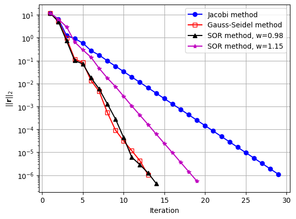
We have two main observations:
The Gauss-Seidel method has a better performance than the Jacobi method (lower iterations to reach the same accuracy).
The relaxation coefficient in the SOR method has a large impact on the method’s performance.
Exercise: Repeat the same experiment for other linear systems, specifically for larger ones. Can you confirm the above observations?