18. Solution of non-linear equations and systems#
Saleh Rezaeiravesh, saleh.rezaeiravesh@manchester.ac.uk
Department of Mechanical and Aerospace Engineering, The University of Manchester, Manchester, UK
18.1. Intended Learning Outcomes#
After reading and running this notebook, the students should be able to:
Implement simple iteration and Newton-Raphson’s methods in Python for solving non-linear equations with a single unknown.
Implement Newton-Raphson’s method in Python to solve a system of non-linear equations.
18.2. Import libraries#
In this notebook, we rely on the methods provided by numpy and numpy.linalg. We also use matplotlib for making plots.
import numpy as np
import numpy.linalg as la
import matplotlib.pyplot as plt
18.3. Simple iteration method#
Consider we want to solve \(f(x)=0\), where \(f(x)\) is a non-linear function of the single unknown variable \(x\). If we can write this equation as \(x = g(x)\), then the simple iteration method can be applied. To update the solution at the \(k\)-th iteration, we have,
To ensure convergence, at each iteration, we should have,
Below, we demonstrate how to write a python function for the simple iteration method. The iterations stop when \(|x^{(k)}-x^{(k-1)}|<\varepsilon\) for a given small tolerance \(\varepsilon\).
Example: Find the solution(s) of the following non-linear function over \(x\in[-2.,0]\) using the simple iteration method:
First, let’s plot this function and see how many roots it has (this is for demonstration purposes; otherwise, this is not a required/possible step in practice):
def f(x):
    return 2*x**2.-x+3*x*np.sin(4*x)-1.5
X = np.linspace(-2,0,200)
plt.plot(X,f(X))
plt.hlines(0.0,np.min(X),np.max(X),linestyles='dashed',colors='r')
plt.show()
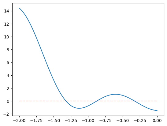
This function has 3 roots over \([-2,0]\).
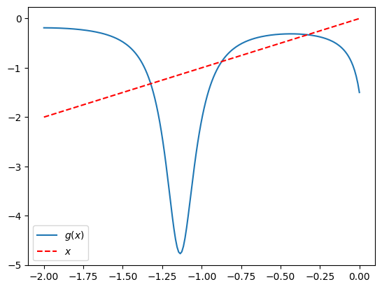
To apply the simple iteration method, we need to re-write the original equation in the form of \(x=g(x)\):
The function \(g(x)\) is implemented below:
def g(x):
    return 1.5/(2*x-1+3.*np.sin(4.*x))
plt.plot(X,g(X),label=r'$g(x)$')
plt.plot(X,X,'--r',label=r'$x$')
plt.legend(loc='best')
plt.show()
Now, we can write the function simpleIter with two input arguments: the initial guess x0 and convergence tolerance eps:
def simpleIter(x0,eps):
    """
    Simple iteration method to solve x=g(x)
    """
    err = 10*eps   #initial error: arbitrarily value larger than eps    xold = x0
    xold = x0

    k=0            #iteration count
    errA = []      #list to collect the iterations error
    while err > eps:
       x = g(xold)       #update the solution
       err = abs(x-xold) #compute the error
       errA.append(err)
       xold = x
       k += 1

    return x,k,errA
This function can be called for different initial guesses:
x, k, errA = simpleIter(x0=-0.8,eps=1.e-8)
print('Converged x:', x)
print('Number of iterations:', k)
Converged x: -0.3289008177497181
Number of iterations: 19
For the computed solution, the reduction of the errors can be plotted:
plt.semilogy(np.arange(1,len(errA)+1),errA,'-xr')
plt.xlabel('Iteration')
plt.ylabel(r'$|x^{(k)}-x^{(k-1)}|$')
plt.show()
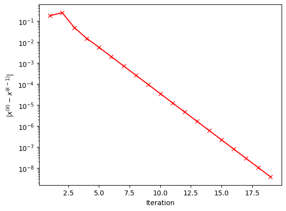
What can you say about the convergence rate of the simple iteration method?
Exercise: Try different values of initial guess x0 and see how many of the three zeros of the above \(f(x)\) can be computed by the simple iteration method. Can you motivate your observations.
Exercise: Can you modify simpleIter(x0,eps) to check the convergence condition \(|g'(x^{(k-1)})|<1\)?
18.4. Newton-Raphson method#
To solve the non-linear equation \(f(x)=0\), the Newton-Raphson’s iterations read as,
for \(k=1,2,\cdots\). Starting from an initial guess \(x^{(0)}\), iterations run until \(|x^{(k)}-x^{(k-1)}|<\varepsilon\). Alternatively, we can stop the iterations when \(|r^{(k)}|<\varepsilon\), where the residual at the \(k\)-th iteration is \(r^{(k)} = f(x^{(k)})\).
Example: Find the solution(s) of the following non-linear function over \(x\in[-2.,0]\) using the Newton-Raphson’s method:
First, we write a function that returns the values of \(f(x)\) and its derivative, \(f'(x)\), for any input value of \(x\):
def f_df(x):
    f = 2.*x**2.- x + 3*x*np.sin(4*x) - 1.5
    df = 4.*x - 1 + 12*x*np.cos(4*x) + 3*np.sin(4*x)
    return f,df
def newtonRaphson(x0,eps):
    """
    Newton-Raphson method to solve f(x)=0
    """
    err = 10*eps   #initial error: arbitrarily value larger than eps
    xold = x0

    k = 0   #iteration count
    errA = []      #list to collect the iterations error
    while err > eps:
        f, df = f_df(xold)    #f and f' at xold
        x = xold - f/df       #update the solution
        err = abs(x-xold)     #update the error
        errA.append(err)
        xold = x
        k += 1

    return x,k,errA
This function can be called for different initial guesses:
x,k, errA = newtonRaphson(x0=-.1,eps=1e-6)
print('Converged x:', x)
print('Number of iterations:', k)
Converged x: -0.32890081876610844
Number of iterations: 5
For the computed solution, the reduction of the errors can be plotted:
plt.semilogy(np.arange(1,len(errA)+1),errA,'-ob')
plt.xlabel('Iteration')
plt.ylabel(r'$|x^{(k)}-x^{(k-1)}|$')
plt.show()
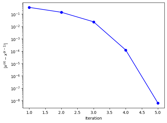
What can you say about the convergence rate of the Newton-Rapshon method?
Exercise: Try different values of initial guess x0 and see how many of the three zeros of the above \(f(x)\) can be computed by the Newton-Raphson method. Do you think the Newton-Raphson’s method is better than the simple iteration method? Why?
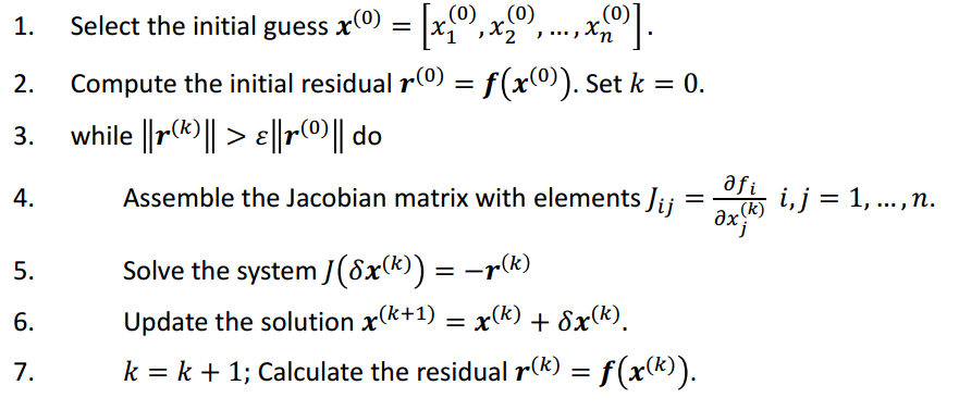
18.5. Solving systems of non-linear equations#
Consider the following system of non-linear equations
We can adopt the following algorithm based on the Newton-Rapshon’s method to solve this system and find \(\mathbf{x}=[x_1,x_2,\cdots,x_n]^T\).
Example: Below, we demonstrate the implementation of this algorithm for the following system of two non-linear equations:
First, we implement the following function to compute \(f_1(x_1,x_2)\), \(f_2(x_1,x_2)\), and their analytical derivatives with respect to \(x_1\) and \(x_2\). Input to these functions is an array of size 2: \(\mathbf{x}=[x_1,x_2]\).
def f1(x):
    return 9.*x[0]**2.*x[1] + 4.*x[1]**2. - 36.

def df1(x):
    df1dx1 = 18.*x[0]*x[1]
    df1dx2 = 9*x[0]**2. + 8.*x[1]
    return df1dx1, df1dx2
def f2(x):
    return 16.*x[1]**2. - x[0]**4. + x[1] + 1.

def df2(x):
    df2dx1 = -4.*x[0]**3.
    df2dx2 = 32.*x[1] + 1.0
    return df2dx1, df2dx2
The above algorithm is implemented in the following function with two input arguments: x0, initial guess (vector of size 2), and eps, the convergence tolerance (\(\varepsilon\)).
def NRsys(x0,eps):

    xold = x0

    r = np.array([f1(xold),f2(xold)])    #form the initial residual vector
    resid0 = la.norm(r)                  #norm of the initial residual vector
    resid = resid0

    k = 0    #iteration count
    while resid > eps*resid0:
        #Assemble the Jacobian Matrix
        df1dx1, df1dx2 = df1(xold)
        df2dx1, df2dx2 = df2(xold)
        J = np.array([[df1dx1, df1dx2],[df2dx1, df2dx2]])

        #Solve the linear system J delta_x = - r
        delx = -la.inv(J) @ r    #direct inversion (can use any iterative solver)

        x = xold + delx   #update the solution vector

        #compute the residual vector and its norm
        r = np.array([f1(x),f2(x)])
        resid = la.norm(r)

        xold = x
        k += 1

    return x, k
Now, we can call the function by providing the initial guess \(\mathbf{x}^{(0)}=[x_1^{(0)},x_2^{(0)}]\).
x, k = NRsys(x0 = 0.2*np.ones(2),eps=1.e-8)

print('Converged x:', x)
print('Number of iterations:', k)
Converged x: [1.98370873 0.92074264]
Number of iterations: 16
We can simply check if the converged solution \(\mathbf{x}\) satisfy both equations in the system:
print('f1(x1,x2) at converged x:',f1(x))
print('f2(x1,x2) at converged x:',f2(x))
f1(x1,x2) at converged x: -2.1316282072803006e-14
f2(x1,x2) at converged x: -8.43769498715119e-15